Essentials of Biostatistics

Indian Pediatrics 2001; 38: 43-59

11. Statistical Relationships and the Concept of Multiple Regression

* From the Division of Biostatistics and Medical Informatics, University College of Medical Sciences, Dilshad Garden, Delhi 110 095, India.

** Institute of Cytology and Preventive Oncology, Maulana Azad Medical College Campus, Bahadur Shah Zafar Marg, New Delhi 110 002, India.

Correspondence to: Dr. A. Indrayan, Professor of Biostatistics, Division of Biostatistics and Medical Informatics, University College of Medical Sciences, Dilshad Garden, Delhi 110 095, India.

E-Mail: [email protected]

Relationships are inherent in medicine and health. For example, lung functions are related to height, and greater weight gain in childhood among low birth weight children is associated with a higher chance of myocardial infarction. The methods for studying relationships are different for qualitative variables than for quantitative variables. You know by this time that a variable is considered quantitative when it is measured on a metric scale (continuous or discrete), whereas variables on nominal and ordinal scales as well as those that have broad categories on a metric scale are considered qualitative for most statistical purposes(1).

There are two aspects in the study of relationships. One is the form or type of relationship and the other is the strength of relationship. The strength is generally measured by correlation in quantitative type of variables and by association in qualitative type. For example, different anthropometric measurements in children such as weight, height, mid-arm and calf circumferences are correlated. Symptoms in children of age 6 months to 1 year such as increased biting, ear-rubbing, decreased appetite for solid foods and mild temperature elevation are associated with teething. Some measures of strength of relationships for both qualitative and quantitative variables are discussed in Section 11.1.

What do we actually mean by form of relationship? The form of relationship between weight gain during pregnancy and birth weight would be able to indicate how much increase in birth weight (y) to expect when the pregnancy weight gain (x₁) is 10 kg in one women opposed to 8 kg in another. This is an example of what is called simple regression in statistical sense because there are a total of only two variables in this case. The variables y and x₁ are called dependent and independent, respectively. Thus, the form of relationship is an expression of quantitative change in one variable per unit change in the other. It becomes from simple to multiple regression when the number of independent variables is more than one. For example, birth weight is also related to the other parameters such as maternal Hb level (x₂) and calorie intake during pregnancy (x₃). The type and expression of the regression may vary depending on the number of independent variables and whether the dependent variable (y) is quantitative or qualitative. These are discussed in Section 11.2. Computation of regressions, especially multiple type, involves intricate mathematical expressions. We avoid discussing these and advise use of computer programs to obtain such regressions. Our emphasis is mainly on the concepts and interpretation of such regressions.

There is another type of relationship that is frequently encountered in the practice of medicine and health. This is between two or more measurements on the same variable obtained on the same subjects. Examples of this are: (i) presence or absence of a disease in a group of children diagnosed by two clinicians, and (ii) measurement by two devices, a newly devised and a conventional, for a nutritional anthropometry, such as mid-arm circum-ference. The problem under study in these situations basically is that of agreement between two or more observers, methods, laboratories, etc. Methods of assessing such agreement in both quantitative and qualitative variables are presented in Section 11.3.

You might be interested in strength of relationship between forced vital capacity (FVC) and height in children of age 6 years, or between type of diarrhea and dehydration status in children. Different types of measures of the strength of relationship can be computed depending upon the nature of the variables involved. For simplicity, we restrict our discussion to the strength between two variables only but consider qualitative as well as quantitative variables. For dichotomous variables, the widely used measure of the strength of association is either relative risk (RR) or odds ratio (OR), depending on whether the design is prospective or retrospective/cross-sectional. These are already discussed in an earlier Article(2). The methods for measuring strength between two polytomous variables are phi coefficient, contingency coefficient and proportional reduction in error (PRE). Additional methods are available for ordinal variables. For details refer Freeman(3). We restrict our discussion in this section to strength between two quantitative variables. The following paragraphs contain an explanation of methods of different types, their interpretation, and the statistical test of their significance.

Suppose there exists a correlation between plasma fibronectin and birth weight in healthy new-borns and is reported to be 0.69, i.e., r = 0.69. What does it mean? The meaning of such correlation and its computation is explained below. For actual computation of correlation, statistical packages can be used.

We discussed earlier(1) about the variability in a single measurement. Standard deviation measures this variability. The variation in the values of one variable in relation to the other is of special interest in medicine and health. One such relationship was depicted earlier(4) through a scatter diagram of oxygen saturation (%) with heart rate in asphyxiated new-borns at birth. Compared to the term variance in one variable, variation in relationship between two variables depends on a quantity called covariance. This is the sum of the products of (x – "x) and (y – "y), which are deviations from the respective mean. However, the covariance primarily measures the direction of relationship. The exact magnitude of the relationship depends also on the magnitude of variation in individual variables, i.e., on the variance in x and in y. These can be measured by Öå(x – "x)2 and Öå(y – ""y)² (numerators in the respective SDs). To make the covariance independent of such variation, it is divided by the product of these numerators of respective SDs. This gives the formula for correlation coefficient as follows.

Product-moment correlation coefficient:

       å(x – "x) å(y – ""y)
r = –––––––––––––––––– [1]
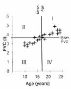
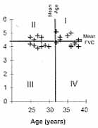
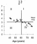
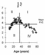
     Öå(x – "x)² Öå(y – ""y)²

The correlation coefficient thus obtained also becomes dimension-less and very easy to interpret. This actually is a measure of linear correlation. Linear is a form of relationship that we discuss in the next Section. For the time being, note that correlation measures the strength of that part of relationship between x and y that can be explained by a straight-line. As there are many types of correlation, this r is sometimes specified as the product-moment coefficient of correlation. The name arises from the numerator, which we have called covariance, but is also called product-moment.

The correlation coefficient (r) is a pure number without any unit and ranges from –1 to +1. A value close to zero indicates that the two variables are linearly un-correlated. That is, a change in the value of one is not accompanied by any linear change in the other. The scatter, then, would be nearly a horizontal (or a vertical) line with no slope. None is linearly affected or affected by the other. But a zero correlation can sometimes arise in the case of clear relationship of nonlinear type. Consider the scatter diagram in Fig. 1 between age x and forced vital capacity (FVC) y. Quadrants I, II, III, IV are drawn by lines corresponding to the mean of x and mean of y in each case. FVC is increasing as age increases from 10 to 24 years (Fig. 1a). This is an indication of positive correlation between x and y. FVC is neither increasing nor decreasing when age is between 25 and 39 years (Fig. 1b). This is an example of almost zero correlation. In Fig. 1c, FVC decreases as age increases from 40 to 79 years. This inverse relationship yields a negative correlation. Fig. 1d shows the relationship when all ages between 10 and 79 years are considered together. This will give a small value of correlation coefficient because there is no clear linear relationship. This should not be construed to mean that there is no relationship between age and FVC. The relationship is in fact strong and can be expressed by a form other than a straight line. A perfect r = ±1 would mean that the scatter of y with x forms an exact straight line with some slope. This slope could be small or large. Such perfect correlation seldom occurs in health and medicine. Note that the points are widely scattered around a line in case of weak correlation but very close to a line in case of strong correlation.

Spurious or Nonsense Correlation: During the months of August and September, there is high birth rate in Delhi and high pollen density in Boston area. The reasons for these are very different and unrelated. The correlation between birth rate of Delhi and pollen density of Boston area over a 12-month period may turn out to be high but such a correlation has no meaning. A correlation arising because of intervention of a third, irrelevant, variable is called a spurious or nonsense correlation. Also, very few correlations can be considered to indicate a cause-effect type of relationship. Such relationships will be discussed in a future Article of this series.

Fig. 1. Scatter of forced vital capacity (FVC) by age. (a) For the age group (10-24) years. (b) For the age group (25-39) years. (c) For the age group (40-79) years. (d) Combined for all the age groups.

Statistical Significance of r: A correlation coefficient r is called statistically significant when the probability of it being zero in the population (H₀: r = 0) is less than 0.05 or any other such predetermined level of significance. The test criterion for this is:

     r Ö n – 2
t = ––––––––                                                         [2]
     Ö 1 – r²

This follows Student’s t-distribution with (n – 2) df. The test is valid provided at least one of the variables follows a Gaussian pattern. If this condition is not met, it is advisable to use rank correlation that we describe in the next paragraph.

Example 1: Suppose the correlation between erythrocyte sedimentation rate and weight length index in children is r = 0.55 in a sample of size n = 66. Its statistical significance can be assessed by

     0.55 Ö 66 – 2
t = –––––––––––– = 5.268
        Ö 1 – 55²

For this value of t, P <0.001 using standard t-table at 64 df. Thus, this correlation is almost surely not zero in the target population of such subjects from which this sample of 66 was randomly chosen.

In some cases, x and y clearly increase or decrease together but the relationship is not necessarily linear. This is called a monotonic relationship. The dependence of height on the age of children is an example of such a relationship. The linearizing effect of the product-moment correlation coefficient in such cases amounts to oversimplification of the relationship. An alternative is the rank correlation. For this, the values of x and y are separately ranked from 1 to n in increasing order of magnitude. Rank correlation is the ordinary product-moment correlation coeffi-cient between ranks of x and ranks of y but the formula simplifies to the following.

            6 å d²
rs = – ––––––––– , [3]
           n (n² – 1)

where d = (rank of y – rank of x) and the summation is over all n pairs of observations. Equal ranks are assigned to the tied observations if any.

Example 2: Suppose we have weights and heights of eight children as shown in Table I. The differences d (= rank of weight – rank of height) are also shown. This gives å d² = 0.5 and

              6 X 7.50
r_s = 1 – –––––––– = 0.911 ,
               8 X 63

The ordinary product-moment correlation coefficient between weight and height in this example is 0.962. In this case the rank correlation is less than the product moment correlation, but the rank correlation sometimes can overrate the strength of the relationship because it partially disregards the actual magnitude of x and y.

Statistical Significance of r_s : The full name of the rank correlation coefficient is Spearman’s rank correlation. This explains our subscript S in r_s . This is a nonparametric procedure and the test of its statistical significance does not require a Gaussian pattern of either x or y. This correlation is thus preferable when the distribution pattern of both x and y is far from Gaussian. For samples of 10 or fewer pairs, the minimum values of r_s for different significance levels are available in biostatistics books(5). For n ³ 11, the Gaussian pattern holds reasonably well and the Student’s t-test (equation [2]) used for r can be used for r_s .

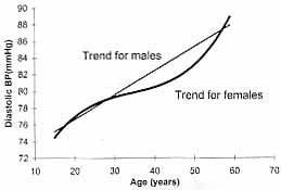
The observed correlation between two variables x and y can be adjusted for one or more other variables that influence their relationship. Correlation after such an adjust-ment is called partial correlation coefficient. The correlation between child’s blood pressure (BP) and mother’s BP after adjusting for father’s BP is an example of this type of correlation. For strange reasons, use of partial correlation coefficient has not become popular in health and medicine. Statistical packages can be used to calculate this type of correlation also.

The exact form of relationship is required to answer the question "How much does one variable change for a specified change in one or more of the other variables?" In an earlier Article(1), we mentioned that there are variables or measurements that are known for the subjects and there are others that are obtained subsequently. In the case of relation-ship between pregnancy weight gain and birth weight, the former is measured a priori and the latter is a subsequent outcome. Pregnancy weight gain represents independent or explanatory variable. The birth weight is the response or dependent variable. The relationship between such variables can be expressed in terms of a mathematical equation called regression. In the pregnancy weight gain and birth weight example, for full-term normal pregnancies, this possibly could be written as:

(Birth weight) = 1.2 + 0.2 X (pregnancy weight gain);                          [4]

6 kg <= pregnancy weight 
gain <=12 kg.

This says that the birth weight increases on average by 0.2 kg for every kg increase in pregnancy weight gain.

The types regressions used in practice are linear, curvilinear and non-linear. Under-standing of the distinction between these types of regressions is important. A study (6) of relationship between the diastolic BP in relation to age in adult males showed straight-line (linear) relationship and that of females curvilinear (Fig. 2). For simplicity, we restrict our discussion to only linear form. This also is the most common form used in practice. Utility and interpretation of linear relationships are discussed under two broad divisions. First involves methods for one quantitative depen-dent variable and the second is for one qualitative dependent variable. If the number of dependent variables is more than one then this falls in the domain of multivariate regression.

Fig. 2. Relationship between diastolic BP and age in adult males and females.

Before we discuss the methods of this type, it is necessary to be clear about the distinction between dependent and independent variables that we explained earlier. The one that is on the left side (birth weight) of the regression equation [4] is dependent and the one on the right side (pregnancy weight gain) is independent. A dependent in one setup can be independent in another setup. For example, birth weight is dependent on parental weight and childhood growth in turn is dependent on birth weight. The independent variables can be more than one, in fact would be more than one in most practical situations. Birth weight depends not just on parental weight but also on nutrition and care during antenatal period. They are not necessarily exclusive of one another.

Simple Linear Regression: The following examples of regression may help to under-stand the concept. Suppose there is a relationship between erythrocyte sedimenta-tion rate (ESR) and a weight-length index (WLI) in obese children (7). If we represent ESR by y and WLI by x, then the scatter plot will be nearly a straight line. The regression equation is

ESR = – 2.98 + 0.14 WLI.

This shows that ESR increases by 0.14 mm/hr on average for one unit increase in WLI. According to this equation, if WLI = 80, then expected ESR is 8.2.

Suppose there is another relationship, now between plasma fibronectin concentration (PFC) and birth weight (BWt) in grams in healthy new-borns(8). This relationship may be written as

PFC = 109.64 + 0.0365 BWt.

The general form of these relationships is represented by best-fitting straight line

y = a + bx.                                  [5]

The value of y on left-hand side of equation [5] is the predicted or estimated value but for simplicity we are not introducing another notation. The best fitting line is the one that is closest to the points in the scatter plot. This is defined as the line that minimizes the sum of the squared distances of the observed values of y from the chosen line. As mentioned earlier, this equation is called a simple regression equation because there is only one independent and one dependent. It is called linear because it represents a straight line. In PFC and BWt example, a = 109.64 is, what is called, the intercept, and b = 0.0365 is, what is called, the slope of the line. Slope is the rate at which y changes for a unit change in x. Intercept is the value of y when x = 0. It may or may not have any biological meaning. For example, in a linear regression of birth weight on amount of bidi smoking by mother, the constant a is the mean birth weight for non-smoking mothers. In this case, the slope b will be negative since birth weight would decline as the smoking increases. In PFC and BWt example, the intercept has no biological meaning as birth weight can not be zero. The constants a and b along with their SE can be obtained from statistical packages for a given data. If the regression coefficient (b) for any variable is zero, then that variable would have no linear influence on y. In case of relationship of intraocular pressure in children on height, b would be nearly zero. In practical situations, it would be unlikely that the b coefficient is exactly zero. Computer programs generally test the significance of regression coefficient using t test of the type used earlier, viz., t = b/estimated SE(b). The significance would indicate presence of some linear relationship between the variables x and y. A prerequisite for this test is the Gaussian pattern of y or large n. For a given value of x, expected y can be predicted using equation [5]. A measure of variability in the predicted y is its standard error (SE). This can also be obtained from the computer packages and can be used to obtain a confidence interval (CI) for predicted y.

Multiple Linear Regression: Multiple linear regression attempts to relate one measurement to more than one explanatory variable. An example is the relationship of body fat (%) with two explanatory variables viz., weight-height index (WT/HT3), where WT is in kg and HT in meters, and triceps skinfold thickness (TSFT) in mm in children given by Frerichs et al.(9). This is

Body fat (%) = 4.67 + 0.85 (WT/HT³) + 0.73 (TSFT).                                [6]

In notations, if y denotes dependent variable, and x₁ and x₂ are two explanatory variables, then multiple linear regression equation for y on x₁ and x₂ is

y = a + b₁ x₁ + b₂ x₂ .

Similarly, regression on K variables is

y = a + b₁ x₁ + b₂ x₂ + . . . + b_Kx_K.                                                         [7]

In this regression, if x₂, for example, increases by unity, and other xs remain the same then estimated y increases by b₂. Thus b_k is the independent contribution of one unit of x_k when other xs remain same. In equation [6], if weight-height index changes from 12.0 to 13.0 and TSFT remains same level at 15.0 mm then expected change in body fat is 0.85%. The usefulness of a regression equation to predict y can be checked by an F-test.

F-test was introduced in the previous Article(10) for comparison of several means using ANOVA procedure. In that case, the total sum of squares (TSS) is broken into between-groups sum of squares and within-groups or residual sum of squares. The results of multiple regression are also sometimes summarized in an ANOVA format with TSS broken down into regression sum of squares and residual sum of squares.

Apart from F-ratio, the other quantity that is computed in this set-up is the coefficient of determination R². This is the fraction of the total variation in y that is accounted for by the fitted regression model and varies from zero to one. For example in equation [6], R² = 0.69 would indicate that 69% of total variation in body fat is explained by weight-height index and triceps skinfold thickness. This is useful in assessing the adequacy of the computed relationship. The other method used to assess the adequacy is the residual plot. Residual is the difference between the observed value and the predicted value of y as per the regression equation. Suppose for a child whose weight is 44.6 kg and height is 1.53 meters, weight-height index is 12.45, TSFT is 15.3 mm and the actual body fat is 27.8%. Then the predicted body fat per cent from equation [6] is 26.4. The residual is 27.8 – 26.4 = 1.4 per cent. A regression model is considered a good fit if such residuals are small for most values of the explanatory variables.

Some Remarks on Regression Models: (i) A simple linear regression is the most common form of regression. This is validated only when the dependent variable tends to rise or fall with a uniform rate with increasing value of the regressor x. (ii) The regression of y on x is not the same as that of x on y. (iii) The predicted value of y will be the "best" that the regression model can predict, but it may still be far from reality. The practical utility of the model depends on the proper choice of regressors. These should be such that they include all those that influence the outcome y. At the same time, they should not be highly correlated amongst themselves. (iv) A regression model can be validly used to predict the level of the response variable only for values of explanatory variable that fall within the range actually used to derive the regression equation. For example, see equation [4] where the eligible values of the explanatory variable are explicitly specified. (v) The basic requirement of F and t tests in the context of regression is that the residuals: (a) have a Gaussian pattern, (b) statistically independent of one another and (c) have the same variance for each values of x. (vi) The practical utility of the model is greatly diminished if one is not able to test its statistical significance, and this can happen if the assumptions are violated.

The steps in fitting regression for quantitative variables are: (a) identification of the dependent variable, and (b) of the regres-sor variables, (c) specification of the form of regression (linear, curvilinear, or nonlinear) that you want to investigate, (d) estimation of the regression coefficients, (e) test of good-ness of fit of the model, (f) significance of individual regression coefficients, and (g) examination of the residuals for validity of the assumptions. Last three steps decide whether or not the fit is adequate.

A model is considered better when it contains a small number of regressors but gives a sufficiently large value of R2. Generally, a value of 0.70 is considered desirable, 0.80 good and 0.90 excellent. The success in achieving this depends on the proper choice of regressors. Most statistical softwares do this easily. It is possible to start with a large number of regressors and ask the computer program to include only those that contribute significantly to R². A statistical procedure, similar to the F-test for ANOVA, is available to test the statistical significance of R² as well as of addition to R² made by any additional variable. The selection can be done by different approaches viz., forward selec-tion, backward elimination and stepwise. In the forward selection, the coefficient of a variable with highest statistical significance (i.e., with least P-value) is entered first, and then those that are significant in diminishing order are entered subsequently. In the case of backward elimination, all explanatory vari-ables are included in the first step and then deleted one at a time starting from the least significant. In both procedures above, a variable once entered continues to remain in the model and a variable deleted remains excluded. The third algorithm, called step-wise, re-examines the utility of variables already entered and deletes those that become not significant after addition of other explanatory variables.

The proportion of total variation explained by the regressors, R², which we earlier called the coefficient of determination, has a positive square root, R, but has no particular name when the relationship is nonlinear. However, it is called the coefficient of multiple correlation when the relationship is linear and the number of regressors is more than one. In this case, no meaning can be attached to the direction of the correlation and thus R is never negative. When the relationship is linear and when there is only one regressor, then R² = r².

The method used for qualitative dependent is logistic regression. It can have a dichotomous or polytomous categories. The dichotomous is the type that has yes or no, disease or non-disease type of categories. As there are only two possible responses, this type is also called binary.

Logistic Regression: Occurrence of diarrhea deaths in hospitalized children is dichotomous (yes or no). This may be investigated to depend on, say, infections such as pneumonia, septicemia or meningitis (yes or no), severe wasting (<=50% weight for age or >50%) and extent of stunting (height-for-age as percent of expected height). A binary variable is also obtained when a continuous variable is dichotomised, such as birth weight <2.5 kg and =>2.5 kg. In all such cases, the dependent variable is actually the proportion or probability of subjects with the specific outcome. We have been denoting this probability by p for population and by p for proportion in the sample.

It has been observed that the results lend themselves to easy and useful interpretation if the binary dependent is transformed to logistic of p as

            p
l = ln –––––                                                               [8]
        1 – p

If the probability of complication in mumps cases is 0.02, its logistic is ln (0.02/0.98) = –3.892. Note that p/(1 – p) represents the odd for presence of the response in the subjects. Logistic transformation [8] helps to linearize the relationship between dependent p and explanatory variables, whereas the relation-ship between un-transformed p and other factors is generally non-linear, taking the shape of sigmoid S in place of a line. The logistic relationship recognizes that the probability p is always between zero and one. Classical regression fails to ensure this restriction. The probability is given by p = 1/(1 +e^–l ) and is directly obtained from [8]. The functional form of relationship between l and its possible predictors is called a logistic regression or logistic model. For a simple case with one predictor, say x₁, which is a binary predictor with value one for exposed subjects and value zero for unexposed subjects, the logistic model is

l = b₀ + b₁ x₁.                                                        [9]

The coefficients b₀ and b₁ are intercept and slope respectively. Since the dependent variable in [9] is logistic (p) and p/(1 – p) is odd, the regression coefficient b₁ is the log of ratio of odd for exposed subjects (x₁ = 1) to odd for unexposed subjects (x₁ = 1). Thus b₁ is the log-odds ratio. We explain this with the help of an example.

Example 3: Consider the data given in Table II for the relationship between low birth weight (BW <2500 g) and low maternal height (MHt <145 cm). The proportion (p) of LBW among small mothers is 30/80 = 0.3750 and among ‘normal’ mothers is 222/901 = 0.2464. Since odd = p/(1 – p), the odd of LBW among small mothers is 0.3750/(1 – 0.3750) = 0.600 and among ‘normal’ mothers is 0.2464/(1 – 0.2464) = 0.327. The ratio of these two odds is 0.600/0.327 = 1.835. The logarithm of this OR is ln(1.835) = 0.607. A logistic model obtained for this data using a computer package can be written as

Logistic (p) = 1.118 + 0.607 (MHt);                               [10]

(SE (b₁) = 0.243; t = 2.49, P = 0.0124);

where p is the proportion of low birth weight (LBW) newborns and LBW cases are coded as 1 and nonLBW as 0. The predictor, MHt less than 145 cm is coded as 1 else 0. Note that the coefficient 0.607 is the log-odds ratio. The anti-log of 0.607 gives the odds ratio (OR) as e^0.607 = 1.835. This says that there is nearly 2-fold risk for a newborn to be an LBW when maternal height is less than 145 cm as compared to height more than or equal to 145 cm. This OR is significant as evaluated from t-test since P <0.05.

Let us explain further how the coefficient 0.607 is the log of odds ratio. Under the binary coding scheme as adopted in this example, MHt = 1 when maternal height is less than 145 cm. For these women, equation [10] gives

Logistic (p) = ln [p/(1 – p)] = – 1.118 + 0.607 and odd = p/(1 – p) = e^{–1.118+0.607} and for women MHt = 0, equation [10] gives

Logistic (p) = ln[p/(1 – p)] = – 1.118 and odd = p/(1 – p) = e^–1.118.

Thus, odds ratio = e^{–1.118+0.607} /e^–1.118 = e^0.607 and ln (odds ratio) = 0.607. This is the same as b₁ in equation [9]. It should be now clear that b₁ is the log of odds ratio.

A multiple linear logistic regression takes the form

l = b₀ + b₁x₁ + b₂x₂ + ... + b_K x_K , [11]

if there are K predictors. Computer programs easily provide the values of the coefficients b₀, b₁, b₂, ... , b_K . The coefficient b_k is interpreted as log-odds ratio of the variable x_k when the other bs remain same. The interpretation bs is easy and direct when xs are binary that take value zero for absence and one for presence of the corresponding factor. If there are more than two categories, these categories can be converted to meaning-full contrasts that take on value zero or one. Using the equation [11], the probability of subjects with specific outcome can be calculated. In diarrhea example, probability of fatal diarrhea can be estimated for each subject according to the binary response of different independent variables such as, infection, wasting and stunting.

Meaning and Interpretation of a Logistic Model: Suppose we have a logistic regression model of fatal diarrhea on risk factors in hospitalized children(11). The model reported in this case is

Logistic (p) = 0.42 (PD) + 1.18 (WAG) + 0.66 (HAG) + 1.54 (MAI),

where p is proportion of deaths due to diarrhea among exposed or unexposed subjects for different predictors, PD is the protracted diarrhea, WAG is weight for age, HAG is height for age and MAI is major associated infection. The binary-coding pattern adopted for different variables is as follows. Of the total diarrhea cases, death is coded as 1 and the children that are discharged are coded as 0. PD of more than 14 days is coded as 1 else 0, WAG less than or equal to 50% is coded as 1 else 0, HAG less than or equal to 85% is coded as 1 else 0, and MAI presence is coded as 1 and absence 0.

In this example, all the explanatory variables, PD, WAG, HAG and MAI are in binary form and their coefficients bs can be directly interpreted as log-odds ratios. For example, 1.54 is the log-odds ratio for MAI. This can be converted to odds ratio as e^1.54 = 4.7. This is because mathematically the anti-log is in exponential form. This odds ratio says that presence of major associated infection in diarrhea admissions will entail nearly 5-fold risk for a fatal outcome as compared to absence of that infection when PD, WAG and HAG remain same. Odds ratios thus obtained from multiple logistic regression are called adjusted odds ratios. If we do not adjust for any of the variables, the odds ratio is of crude nature and its magnitude may differ from that of adjusted one. Adjustment for variable or variables that confound the relationship between regressor and dependent is essential when no matching is done between cases and controls.

A logistic coefficient b close to zero implies that the corresponding independent or explanatory variable is not a good predictor. Whether or not log odds ratio is significantly different from zero (or odds ratio is different from 1.0) can be tested. One method is to refer [b/SE(b)] to the standard Gaussian table just as in the case of classical regression. This requires a large sample size. The CI for log-odds ratio [b+SE(b)]. Non-significance of odds ratio can also be noticed from its CI if it includes the value 1.0.

Examining the Adequacy of the Model: For assessing the adequacy of a logistic regression model, an approach called "log-likelihood" is used. The likelihood (L) is the probability of obtaining the values observed in the sample when the model is correct. A probability is necessarily a small number – less than one. It is helpful to use –2 lnL instead of L because: (a) this transformation inflates the value and (b) the distribution of –2 lnL for large n can be approximated by chi-square under H₀ in fairly general conditions. The H0 in the case of logistic is that there is no relationship between the dependent probability and the explanatory variables. If H₀ is true, then b₁, b₂ , ... , b_K all should be close to zero. Statistical packages give the value of –2 ln L for a fitted model that can be compared with values in standard chi-square table to assess statistical signifi-cance.

Different approaches discussed for selection of appropriate independents in the case of classical regression can also be used for logistic regression. The criterion of – 2 ln L has an analogy with (1 – R²), which is used for classical regression. The variables that do not significantly decrease –2 ln L do not find a place in the model in the case of forward selection approach. For testing significance, the difference between –2 ln L without and with the term in question is referred to c² with one df. The procedure of backward selection stops when further deletion would not significantly reduce –2 ln L. The stepwise procedure stops when neither deletion nor addition significantly alters –2 ln L.

We discussed earlier in this section about the classical regression for the case when y and all of xs are quantitative. When y is qualitative and dichotomous (xs can be qualitative or quantitative or a mixture), the relationship is studied in terms of logistic regression. When dependent is quantitative and the independents are qualitative, this becomes an ANOVA setup. In that sense, ANOVA too is a special form of regression. When dependent is quantitative and independents are a mixture of qualitative and quantitative variables, the setup is called analysis of covariance (ANCOVA). This essentially is ANOVA in which differences between groups (qualitative variable) are tested after controlling for quantitative variables, now called covariates. The response y is statistically adjusted in this case to account for group differences in covariates. This set-up is slightly more complex and is outside the scope of the present series.

The science of medicine is growing at a rapid rate. New instruments are invented and new methods discovered that measure anatomical and physiological parameters with better accuracy and precision, and at a lower cost. Emphasis is on simple, non-invasive, safer methods that require smaller sampling volumes and can help in continuous monitoring of patients when required. Acceptance of a new method depends on convincing demonstration that it is nearly as good as, if not better than, the established method.

Irrespective of what is being measured, it is highly unlikely that the new method would give exactly the same reading in each case as the old method even if they were equivalent. Some difference would necessarily arise. How do we decide that the new method is interchangeable with the old? The problem is described as one of agreement. This is different from evaluating which method is better. The assessment of "better" is done with reference to a "gold standard". Assessment of agreement does not require any such standard.

The term agreement is used in several different contexts. We restrict it to the setup where a pair of observations (x,y) is obtained by measuring the same characteristic on the same subject by two different methods, two different observers, two different laboratories, two anatomical sites, etc. The measurement could be qualitative or quantitative. The method of assessing agreement in these two cases is different.

The problem of agreement in quantitative measurements can arise in at least five different types of situations. (a) Comparison of partent-reported values with the instrument-measured values, e.g., urine frequency-volume by patient questionnaire and frequency-volume chart. (b) Comparison of measurements at two different sites, e.g., paracetamol concentration in saliva with that in serum. (c) Comparison of two methods, e.g., bolus and infusion methods of estimating hepatic blood flow in patients with liver disease. (d) Comparison of two observers, e.g., duration of electroconvulsive fits reported by two psychiatrists on the same group of patients, or of two laboratories when, for example, splits of the same sample are sent to two laboratories for analysis. (e) Intra-observer consistency, e.g., measurement of anterior chamber depth of an eye segment two times by the same observer using the same method – to evaluate reliability of the method.

In the first four cases, the objective is to find whether or not a simple, safe, less expensive procedure can replace an existing procedure. In the last case, it is evaluation of the reliability of the method.

The statistical problem in all these cases is to check whether or not a y = x type of relationship exists in individual subjects. This may look like a regression setup y = a + bx with a = 0 and b = 1, but that really is not so. The difference is that, in regression, the relationship is between x and the average of y. In agreement setup, the concern is with individual values and not with averages. Nor should agreement be confused with high correlation. We illustrate this with the help of an example.

Example 4: Suppose the hemoglobin (Hb) levels in g/dl reported for the same group of six children are 11.7, 12.1, 13.8, 12.4, 11.8, 13.0 and 11.5, 12.0, 13.9, 12.6, 12.1, 12.7 from laboratory-1 and laboratory-2, respectively. The two laboratories have same mean (12.5) for these six samples and a very high correlation (r = 0.96). Yet there is not agree-ment in any of the subjects. The difference or error ranges from 0.1 to 0.3 g/dl. This is substantial in the context of the present-day technology. Thus, equality of means and a high degree of correlation are not enough to conclude agreement. Special methods are required. Two approaches are available.

Limits of (Dis)agreement Approach: In this method, the differences d = (x – y) in the values obtained by the two methods or observers under comparison are examined. If these differences are randomly distributed around zero and none of the differences is "large", the agreement is considered good. Note that when the two methods or two observers are measur-ing the same variable, then the difference d is mostly the measurement error. Such errors are known to follow a Gaussian distribution. Thus the distribution of d in most cases would be Gaussian. Then, the limits "d ± 2SD_d are likely to cover differences in nearly 95% of subjects. These are now called the limits of agreement. They are actually limits of disagreement because they show the magnitude of disagreement. If these limits are within clinical tolerance in the sense that a difference of that magnitude does not alter the management of the subjects, then one method can be replaced by the other. The mean difference "d is the bias between the two sets of measurements and SD_d measures the magnitude of random error. For further details, see Bland and Altman(13).

Example 5: Consider the data given by Chawla et al.(14) on systolic BP reading derived from the plethysmographic waveform of a pulse oximeter. This method could be useful in a pulseless disease such as Takayasu syndrome. The readings were obtained at the: (a) disappearance of the waveform on the pulse oximeter on gradual inflation of the cuff, and at the (b) reappearance on gradual deflation. In addition, BP was measured in a conventional manner by monitoring the Korotkoff sounds. The study was done on 100 healthy volunteers. The readings at disappearance of the waveform were observed to be generally higher and at reappearance generally lower. Thus the average (AVRG) of the two is considered a suitable value for investigating the agreement with the Korotkoff readings. The results are given in Table III. Despite means being nearly equal and r very high, the limits of disagree-ment show that a difference of nearly 13 mmHg can arise between the two readings on either side (pulse oximetry can give either less or more than the Korotkoff readings). These limits are further subject to sampling fluctuation, and the actual difference in individual cases can be higher. Now it is for the clinician to decide whether a difference of such magnitude is tolerable. If it is, then the agreement can be considered good and pulse oximetry readings can be used as a substitute for Korotkoff readings, otherwise not. Thus, the final decision is clinical rather than statistical.

Intraclass Correlation: This is the strength of linear relationship between subjects belonging to the same class or the same subgroup or the same family. In the agreement set-up, the two measurements obtained on the same subject by two observers or two methods is a sub-group. If they agree, the intraclass correlation will be high. The computation of this correlation is slightly different from that of product-moment correlation coefficient (r). The formula of intraclass correlation (rI) coefficient (for a pair of readings) is

         2 X å_i (x_i1 – #x ) (x_i2 – #x )
rI #= ––––––––––––––––––––-–--– , [12]
       å_i (x_i1 – #x )² + å_i (x_i2 – #x )²

where x_i1 is the measurement on the ith subject (i = 1, 2, ... , n) when obtained by the first method or the first observer, x_i2 is the measurement on the same subject by the second method or the second observer, and "x is the overall mean of all 2n observations. Note the difference in the denominator compared with formula of r in equation [1].

This was calculated for the systolic BP data described in Example 5 and was found to be r_I = 0.87. A correlation more than 0.75 is generally considered good agreement. Thus, in this case, the conclusion on the basis of the intraclass correlation is that the average of readings at disappearance and appearance of the waveform in pulse oximetry agrees fairly well with the Korotkoff reading. This may not look consistent with the limits of disagreement that showed a difference up to 13 mmHg between the two methods. The two approaches of assessing agreement can sometimes lead to different conclusions. The merits and demerits of the two approaches are discussed by Indrayan and Chawla(15).

Assessing optical disc characteristics by two or more observers, results of Lyme disease serological testing by two or more laboratories, and comparison of X-ray images with Doppler images are examples of the problem of qualitative agreement. The objective is to find the extent of agreement between two or more methods, observers, laboratories, etc. In some cases, for example in comparison of labora-tories, agreement has the same interpretation as reproducibility. In the case of comparison of observers, it is termed interrater reliability.

Consider the data in Table IV on lesion in X-rays read by two radiologists. The two observers agree on a total of 40 cases in this example. This is the sum of the frequencies in the leading diagonal cells. In the other 20 cases, the observers do not agree. Apparently, agreement = 40/60 = 66.7%. But part of this agreement is due to chance, which might happen if both are dumb observers and randomly allocate subjects to present and absent categories. This chance agreement is measured by the cell frequencies expected in the diagonal when the observers’ ratings are independent of one another. The expected frequencies are obtained by multiplying the respective marginal totals and dividing by the grand total. This procedure is the same as used earlier to calculate chi-square(2).

For the data in Table IV, the chance-expected frequencies are 36 ´ 42/60 = 25.2 and 24 ´ 18/60 = 7.2 in the two diagonal cells. The total of these two is 32.4. Agreement in excess of chance is in only 40 – 32.4 = 7.6 cases. The maximum possible value of this excess is 60 – 32.4 = 27.6. A popular measure of agreement is the ratio of the observed excess to the maximum possible excess – in this case 7.6/27.6 = 0.275 or 27.5%. Thus, the two observers in this case do not really agree much on rating of X-rays for the presence or absence of the lesion.

Kappa statistic: In terms of notations, the foregoing procedure to measure agreement between qualitative characteristics is given by

                                å O_ii – å (O_i .O._i /n)
Kappa Statistic: k = ––––––––––––––––––– ,                       [13]
                                   n – å (O_i .O._i /n)

where O_ii is the cell frequency in the ith row and ith column (diagonal element), Oi. is the marginal total in the ith row, O.i is the marginal total in the ith column, and n is the grand total. The first term in the numerator is the observed agreement and the second term is the chance agreement. Thus, the numerator is the agree-ment in excess of chance. The denominator is its maximum possible value. This k is for general I ´ I table; i.e., the rating is not necessarily restricted to the present-absent type of dichotomy but could also be into three or four or a larger number of categories.

Example 6: Maternal and cord blood samples from 174 pregnant women of middle socio-economic group were tested for hemagglutina-tion inhibition (HI) antibodies against measles in Delhi during October 1993 to January 1995(16). The agreement in detection of antibodies at different titre groups is given in Table V. In this case,

     (42+67+8)–(65x68 /174+93x92 /174+16x14/ 174)
k = –––––––––––––––––––––––––––––––––––––––
           174–(65x68 /174+93x92 /174+16x14 /174)

= 41.138 / 98.138 = 0.42.

In this example, the kappa value is 0.42, which is low and indicates a rather poor agreement. A value of k more than 0.7 is generally considered to indicate good agreement.

Kappa is valid for nominal categories only. Ordinal, as in the case of our example, or metric categories are considered nominal by this measure and the order is ignored. The other assumptions are that (a) the subjects are independent; (b) the observers, laboratories, or methods under comparison operate indepen-dently of one another; and (c) the rating categories are mutually exclusive and exhaus-tive. These conditions are easily fulfilled in most practical situations.

The kappa value is +1 for complete agreement and zero if the agreement is the same as expected by chance. However, the value does not become –1 for complete dis-agreement. Thus, it is a measure of the extent of agreement but not of disagreement.

The summary of different methods on relationships and agreement are given in Table VI.

1. Indrayan A, Satyanarayana L. Essentials of Biostatistics: 4. Numerical methods to summarise data. Indian Pediatr 1999; 36: 1127-1134.

2. Indrayan A, Satyanarayana L. Essentials of Bio-statistics: 9. Statistical inference from qualita-tive data-proportions, relative risks and odds ratios. Indian Pediatr 2000; 37: 967-981.

3. Freeman DH. Applied Categorical Data Analy-sis. New York: Marcel Dekker, 1987.

4. Indrayan A, Satyanarayana L. Essentials of Bio-statistics: 5. Graphical methods to sum-marise data. Indian Pediatr 2000; 37: 55-62.

5. Indrayan A, Sarmukaddam S. Medical Bio-statistics. New York: Marcel Dekker, Inc., 2000.

6. Indrayan A, Srivastava RN, Bagchi SC. Age regression of blood pressure in an urban population of age 15-59 years. Indian J Med Res 1972; 60: 966-972.

7. Kasapcour O, Ozdogan H, Yazici H. Obesity and erythrocyte sedimentation rate in children. J Pediatr 1991; 119: 773-775.

8. Yoder MC, Douglas SD, Gerdes J, Kline J, Polin RA. Plasma fibronectin in healthy newborn infants: Respiratory distress syndrome and perinatal asphyxia. J Pediatr 1983; 102: 777-780.

9. Frerichs RR, Harsha DW, Berenson GS. Equations for estimating percentage of body fat in children 10-14 years old. Pediatr Res 1979; 13:170-174.

10. Indrayan A, Satyanarayana L. Essentials of Biostatistics: 10. Statistical inference from quantitative data–comparison of means and other locations. Indian Pediatr 2000; 37: 1210-1227.

11. Sachdev HPS, Kumar S, Singh KK, Satyanarayana L, Puri RK. Risk factors of fatal diarrhea in hospitalized children in India. J Pediatr Gastroenterol Nutr 1991; 12: 76-81.

12. Marquis GS, Habicht J, Lanata CF, Black RE, Rasmussen KM. Association of breastfeeding and stunting in Peruvian toddlers: an example of reverse causality. Int J Epidemiol 1997; 26: 349-356.

13. Bland JM, Altman DG. Statistical methods for assessing agreement between two methods of clinical measurement. Lancet 1986; 1: 307-310.

14. Chawla R, Kumarvel V, Girdhar KK, Sethi AK, Indrayan A, Bhattacharya A. Can pulse oximetry be used to measure systolic blood pressure? Anesth Analg 1992; 74: 196-200.

15. Indrayan A, Chawla R. Clinical agreement in quantitative measurements. Natl Med J India 1994; 7: 229-234.

16. Singh J, Khare S, Prabha S, Chandra R, Jain DC, Bhatia R, Sokhey J. Transplacental transfer of measles antibody in Delhi. Indian Pediatr 1998; 35: 1187-1191.