|
|
|
Indian Pediatr 2011;48:
277-287 |
 |
Receiver Operating Characteristic (ROC) Curve
for Medical Researchers |
|
Rajeev Kumar and Abhaya Indrayan
From the Department of Biostatistics and Medical
Informatics, University College of Medical Sciences, Delhi, India.
Correspondence to: Mr Rajeev Kumar, Department of
Biostatistics and Medical Informatics,
University College of Medical Sciences, Delhi 110 095.
Email:
[email protected]
|
Sensitivity and specificity are two components that measure the inherent
validity of a diagnostic test for dichotomous outcomes against a gold
standard. Receiver operating characteristic (ROC) curve is the plot that
depicts the trade-off between the sensitivity and (1-specificity) across
a series of cut-off points when the diagnostic test is continuous or on
ordinal scale (minimum 5 categories). This is an effective method for
assessing the performance of a diagnostic test. The aim of this article
is to provide basic conceptual framework and interpretation of ROC
analysis to help medical researchers to use it effectively. ROC curve
and its important components like area under the curve, sensitivity at
specified specificity and vice versa, and partial area under the
curve are discussed. Various other issues such as choice between
parametric and non-parametric methods, biases that affect the
performance of a diagnostic test, sample size for estimating the
sensitivity, specificity, and area under ROC curve, and details of
commonly used softwares in ROC analysis are also presented.
Key words: Sensitivity, Specificity, Receiver operating
characteristic curve, Sample size, Optimal cut-off point, Partial area
under the curve.
|
|
D
iagnostic tests play a vital role in modern medicine not only for
confirming the presence of disease but also to rule out the disease in
individual patient. Diagnostic tests with two outcome categories such as a
positive test (+) and negative test (–) are known as dichotomous, whereas
those with more than two categories such as positive, indeterminate and
negative are called polytomous tests. The validity of a dichotomous test
compared with the gold standard is determined by sensitivity and
specificity. These two are components that measure the inherent validity
of a test.
A test is called continuous when it yields numeric
values such as bilirubin level and nominal when it yields categories such
as Mantoux test. Sensitivity and specificity can be calculated in both
cases but ROC curve is applicable only for continuous or ordinal test.
When the response of a diagnostic test is continuous or
on ordinal scale (minimum 5 categories), sensitivity and specificity can
be computed across all possible threshold values. Sensitivity is inversely
related with specificity in the sense that sensitivity increases as
specificity decreases across various threshold. The receiver operating
characteristic (ROC) curve is the plot that displays the full picture of
trade-off between the sensitivity and (1- specificity) across a series of
cut-off points. Area under the ROC curve is considered as an effective
measure of inherent validity of a diagnostic test. This curve is useful in
(i) finding optimal cut-off point to least misclassify diseased or
non-diseased subjects, (ii) evaluating the discriminatory ability
of a test to correctly pick diseased and non-diseased subjects; (iii)
comparing the efficacy of two or more tests for assessing the same
disease; and (iv) comparing two or more observers measuring the
same test (inter-observer variability).
Introduction
This article provides simple introduction to measures
of validity: sensitivity, specificity, and area under ROC curve, with
their meaning and interpretation. Some popular procedures to find optimal
threshold point, possible bias that can affect the ROC analysis, sample
size required for estimating sensitivity, specificity and area under ROC
curve, and finally commonly used statistical softwares for ROC analysis
and their specifications are also discussed.
PubMed search of pediatric journals reveals that ROC
curve is extensively used for clinical decisions. For example, it was used
for determining the validity of biomarkers such as serum creatine kinase
muscle-brain fraction and lactate dehydrogenase (LDH) for diagnosis of the
perinatal asphyxia in symptomatic neonates delivered non-institutionally
where area under the ROC curve for serum creatine kinase muscle-brain
fraction recorded at 8 hours was 0.82 (95% CI 0.69-0.94) and cut-off point
above 92.6 U/L was found best to classify the subjects. The area under ROC
curve for LDH at 72 hours was 0.99 (95% CI 0.99-1.00) and cut-off point
above 580 U/L was found optimal for classifying the perinatal asphyxia in
symptomatic neonates [1]. It has also been similarly used for parameters
such as mid-arm circumference at birth for detection of low birth weight
[2], and first day total serum bilirubin value to predict the subsequent
hyperbilirubinemia [3]. It is also used for evaluating model accuracy and
validation such as death and survival in children or neonates admitted in
the PICU based on the child characteristics [4], and for comparing
predictability of mortality in extreme preterm neonates by birth-weight
with predictability by gestational age and with clinical risk index of
babies score [5].
Sensitivity and Specificity
Two popular indicators of inherent statistical validity
of a medical test are the probabilities of detecting correct diagnosis by
test among the true diseased subjects (D+) and true non-diseased subjects
(D-). For dichotomous response, the results in terms of test positive (T+)
or test negative (T-) can be summarized in a 2×2 contingency table (Table
I). The columns represent the dichotomous categories of true
diseased status and rows represent the test results. True status is
assessed by gold standard. This standard may be another but more expensive
diagnostic method or a combination of tests or may be available from the
clinical follow-up, surgical verification, biopsy, autopsy, or by panel of
experts. Sensitivity or true positive rate (TPR) is conditional
probability of correctly identifying the diseased subjects by test: S N
= P(T+/D+) = TP/(TP + FN); and specificity or true negative rate (TNR) is
conditional probability of correctly identifying the non-disease subjects
by test: SP= P(T-/D-) = TN/(TN + FP). False positive rate (FPR)
and false negative rate (FNR) are the two other common terms, which are
conditional probability of positive test in non-diseased subjects:
P(T+/D-)= FP/(FP + TN); and conditional probability of
negative test in diseased subjects: P(T-/D+)= FN/(TP + FN)
respectively.
Table I


Diagnostic Test Results in Relation to True Disease Status in a 2×2 Table
| Diagnostic test result |
Disease status |
Total |
| |
Present |
Absent |
|
| Present |
True positive (TP) |
False positive (FP) |
All test positive (T+) |
| Absent |
False negative (FN) |
True negative (TN) |
All test negative (T-) |
| Total |
Total with disease (D+) |
Total without disease (D-) |
Total sample size |
Calculation of sensitivity and specificity of various
values of mid-arm circumference (cm) for detecting low birth weight on the
basis of a hypothetical data are given in Table II as an
illustration. The same data have been used later to draw a ROC curve.
Table II


Hypothetical Data Showing the Sensitivity and Specificity at Various Cut-off Points of Mid-arm

Circumference to Detect Low Birth Weight
|
Mid-arm circumference (cm) |
Low birthweight
(<2500 grams) (n=130) |
Normal birth weight
(≥2500 grams) (n=870) |
Sensitivity
= TP/(TP+FN) |
Specificity
= TN/(TN+FP) |
| |
True |
False |
False |
True |
|
|
| |
positive (TP) |
negative (FN) |
positive (FP) |
negative (TN) |
|
|
| ≤8.3 |
13 |
117 |
3 |
867 |
0.1000 |
0.9966 |
| ≤8.4 |
24 |
106 |
26 |
844 |
0.1846 |
0.9701 |
| ≤8.5 |
73 |
57 |
44 |
826 |
0.5615 |
0.9494 |
| ≤8.6 |
90 |
40 |
70 |
800 |
0.6923 |
0.9195 |
| ≤8.7 |
113 |
17 |
87 |
783 |
0.8692 |
0.9000 |
| ≤8.8 |
119 |
11 |
135 |
735 |
0.9154 |
0.8448 |
| ≤8.9 |
121 |
09 |
244 |
626 |
0.9308 |
0.7195 |
| ≤9.0 |
125 |
05 |
365 |
505 |
0.9615 |
0.5805 |
| ≤9.1 |
127 |
03 |
435 |
435 |
0.9769 |
0.5000 |
| ≤9.2 & above |
130 |
00 |
870 |
0 |
1.0000 |
0.0000 |
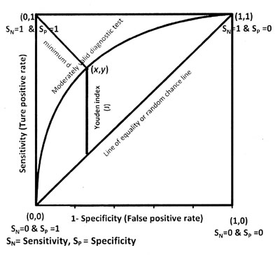
ROC Curve
ROC curve is graphical display of sensitivity (TPR) on
y-axis and (1 – specificity) (FPR) on x-axis for varying cut-off points of
test values. This is generally depicted in a square box for convenience
and its both axes are from 0 to 1. Figure 1 depicts a
ROC curve and its important components as explained later. The area under
the curve (AUC) is an effective and combined measure of sensitivity and
specificity for assessing inherent validity of a diagnostic test. Maximum
AUC = 1 and it means diagnostic test is perfect in differentiating
diseased with non-diseased subjects. This implies both sensitivity and
specificity are one and both errors–false positive and false negative–are
zero. This can happen when the distribution of diseased and non-diseased
test values do not overlap. This is extremely unlikely to happen in
practice. The AUC closer to 1 indicates better performance of the test.
 |
|
Fig. 1 ROC curve and its components. |
The diagonal joining the point (0, 0) to (1,1) divides
the square in two equal parts and each has an area equal to 0.5. When ROC
is this line, overall there is 50-50 chances that test will correctly
discriminate the diseased and non-diseased subjects. The minimum value of
AUC should be considered 0.5 instead of 0 because AUC = 0 means test
incorrectly classified all subjects with disease as negative and all
non-disease subjects as positive. If the test results are reversed then
area = 0 is transformed to area = 1; thus a perfectly inaccurate test can
be transformed into a perfectly accurate test!
Advantages of the ROC Curve
ROC curve has following advantages compared with single
value of sensitivity and specificity at a particular cut-off.
1. The ROC curve displays all possible cut-off
points, and one can read the optimal cut-off for correctly identifying
diseased or non-diseased subjects as per the procedure given later.
2. The ROC curve is independent of prevalence of
disease since it is based on sensitivity and specificity which are known
to be independent of prevalence of disease [6-7].
3. Two or more diagnostic tests can be visually
compared simultaneously in one figure.
4. Sometimes sensitivity is more important than
specificity or vice versa, ROC curve helps in finding the required value
of sensitivity at fixed value of specificity.
5. Empirical area under the ROC curve (explained
later) is invariant with respect to the addition or subtraction of a
constant or transformation like log or square root [8]. Log or square
root transformation condition is not applicable for binormal ROC curve.
Binormal ROC is also shortly explained.
6. Useful summary of measures can be obtained for
determining the validity of diagnostic test such as AUC and partial area
under the curve.
Non-parametric and Parametric Methods to Obtain Area
Under the ROC Curve
Statistical softwares provide non-parametric and
parametric methods for obtaining the area under ROC curve. The user has to
make a choice. The following details may help.
Non-parametric Approach
This does not require any distribution pattern of test
values and the resulting area under the ROC curve is called empirical.
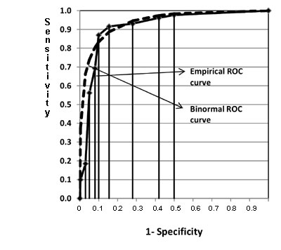
First such method uses trapezoidal rule. It calculates the area by just
joining the points (1-S P,SM) at each interval of the observed
values of continuous test and draws a straight line joining the x-axis.
This forms several trapezoids (Fig 2) and their area can be
easily calculated and summed. Figure 2 is drawn for
the mid-arm circumference and low birth weight data in Table II.
Another non-parametric method uses Mann-Whitney statistics, also known as
Wilcoxon rank-sum statistic and the c-index for calculating area. Both
these methods of estimating AUC estimate have been found equivalent [7].
 |
|
Fig. 2 Comparison of empirical and
binormal ROC curves for hypothetical neonatal data in Table II. |
Standard errors (SE) are needed to construct a
confidence interval. Three methods have been suggested for estimating the
SE of empirical area under ROC curve [7,9-10]. These have been found
similar when sample size is greater than 30 in each group provided test
value is on continuous scale [11]. For small sample size it is difficult
to recommend any one method. For discrete ordinal outcome, Bamber method
[9] and Delong method [10] give equally good results and better than
Hanley and McNeil method [7].
Parametric Methods
These are used when the statistical distribution of
diagnostic test values in diseased and non-diseased is known. Binormal
distribution is commonly used for this purpose. This is applicable when
test values in both diseased and non-diseased subjects follow normal
distribution. If data are actually binormal or a transformation such as
log, square or Box-Cox [12] makes the data binormal then the relevant
parameters can be easily estimated by means and variances of test values
in diseased and non-diseased subjects. Details are available elsewhere
[13].
Another parametric approach is to transform the test
results into an unknown monotone form when both the diseased and
non-diseased populations follow binormal distribution [14]. This first
discretizes the continuous data into a maximum 20 categories, then uses
maximum likelihood method to estimate the parameters of the binormal
distribution and calculates the AUC and standard error of AUC. ROCKIT
package containing ROCFIT method uses this approach to draw the ROC curve,
to estimate the AUC, for comparison between two tests, and to calculate
partial area [15].
The choice of method to calculate AUC for continuous
test values essentially depends upon availability of statistical software.
Binormal method and ROCFIT method produce results similar to
non-parametric method when distribution is binormal [16]. In unimodal
skewed distribution situation, Box-Cox transformation that makes test
value binormal and ROCFIT method perform give results similar to
non-parametric method but former two approaches have additional useful
property for providing smooth curve [16,17]. When software for both
parametric and non-parametric methods is available, conclusion should be
based on the method which yields greater precision to estimate the AUC.
However, for bimodal distribution (having two peaks), which is rarely
found in medical practice, Mann-Whitney gives more accurate estimates
compare to parametric methods [16]. Parametric method gives small bias for
discrete test value compared to non-parametric method [13].
The area under the curve by trapezoidal rule and
Mann-Whitney U are 0.9142 and 0.9144, respectively, of mid-arm
circumference for indicating low birth weight in our data. The SE also is
nearly equal by three methods in these data: Delong SE = 0.0128, Bamber SE
= 0.0128, and Hanley and McNeil SE = 0.0130. For parametric method, smooth
ROC curve was obtained assuming binormal assumption (Fig 2)
and the area under the curve is calculated by using means and standard
deviations of mid-arm circumference in normal and low birth weight
neonates which is 0.9427 and its SE is 0.0148 in this example. Binormal
method showed higher area compared to area by non-parametric method which
might be due to violation of binormal assumption in this case. Binormal
ROC curve is initially above the empirical curve (Fig 2)
suggesting higher sensitivity compared to empirical values in this range.
When (1–specificity) lies between 0.1 to 0.2, the binormal curve is below
the empirical curve, suggesting comparatively low sensitivity compared to
empirical values. When values of (1–specificity) are greater than 0.2, the
curves are almost overlapping suggesting both methods giving the similar
sensitivity. The AUC by using ROCFIT methods is 0.9161 and it standard
error is 0.0100. This AUC is similar to the non-parametric method; however
standard error is little less compared to standard error by non-parametric
method. The data in our example has unimodal skewed distribution and
results agree with previous simulation study [16, 17] on such data. All
calculations were done using MS Excel and STATA statistical software for
this example.
Interpretation of ROC Curve
Total area under ROC curve is a single index for
measuring the performance a test. The larger the AUC, the better is
overall performance of diagnostic test to correctly pick up diseased and
non-diseased subjects. Equal AUCs of two tests represents similar overall
performance of medical tests but this does not necessarily mean that both
the curves are identical. They may cross each other. Three common
interpretations of area under the ROC curve are: (i) the average
value of sensitivity for all possible values of specificity, (ii)
the average value of specificity for all possible values of sensitivity
[13]; and (iii) the probability that a randomly selected patient
with disease has positive test result that indicates greater suspicion
than a randomly selected patient without disease [10] when higher values
of the test are associated with disease and lower values are associated
with non-disease. This interpretation is based on non-parametric
Mann-Whitney U statistic for calculating the AUC.
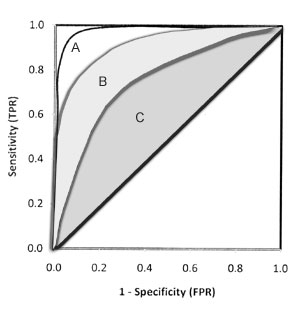
Figure 3 depicts three different ROC
curves. Considering the area under the curve, test A is better than both B
and C, and the curve is closer to the perfect discrimination. Test B has
good validity and test C has moderate.
 |
|
Fig. 3 Comparison of three smooth
ROC curves with different areas. |
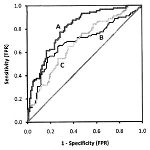
Hypothetical ROC curves of three diagnostic tests A, B,
and C applied on the same subjects to classify the same disease are shown
in Fig 4. Test B (AUC=0.686) and C (AUC=0.679) have
nearly equal area but cross each other whereas test A (AUC=0.805) has
higher AUC value than curves B and C. The overall performance of test A is
better than test B as well as test C at all the threshold points. Test C
performed better than test B where high sensitivity is required, and test
B performed better than C when high specificity is needed.
 |
|
Fig. 4 Three empirical ROC curves.
Curves for B and C cross each other but have nearly equal areas,
curve A has bigger area. |
Sensitivity at Fixed Point and Partial Area Under the
ROC Curve
The choice of fixed specificity or range of specificity
depends upon clinical setting. For example, to diagnose serious disease
such as cancer in a high risk group, test that has higher sensitivity is
preferred even if the false positive rate is high because test giving more
false negative subjects is more dangerous. On the other hand, in screening
a low risk group, high specificity is required for the diagnostic test for
which subsequent confirmatory test is invasive and costly so that false
positive rate should be low and patient does not unnecessarily suffers
pain and pays price. The cut-off point should be decided accordingly.
Sensitivity at fixed point of specificity or vice versa and partial area
under the curve are more suitable in determining the validity of a
diagnostic test in above mentioned clinical setting and also for the
comparison of two diagnostic tests when applied to same or independent
patients when ROC curves cross each other.
Partial area is defined as area between range of false
positive rate (FPR) or between the two sensitivities. Both parametric (binormal
assumption) and non-parametric methods are available in the literature
[13,18] but most statistical softwares do not have option to calculate the
partial area under ROC curve (Table III). STATA software has
all the features for ROC analysis.
Table III


Some Popular ROC Analysis Softwares and Their Important Features
Name of ROC analysis software
|
Methods used to estimate AUC of ROC curve and its |
Comparison of two or more ROC curves |
Partial area |
Important by-products |
| |
variance |
|
Calculation |
Comparison |
|
|
Medcalc software version 11.3; Commercial software trial version
available at: www.medcalc.be |
Non-parametric |
Available |
Not available |
Not available |
Sensitivity, specificity, LR+, LR- with 95% CI at each possible
cut-point |
|
SPSS version 17.0; |
Non-parametric |
Not
available |
Not
available |
Not
available |
Sensitivity and |
|
Commercial software |
|
|
|
|
specificity at each |
| |
|
|
|
|
cut-off point - no 95% Cl |
|
STATA version 11; Commercial software |
Non-parametric Parametric (Metz et al.) |
Available for paired and unpai-red subjects with
Bonferroni adjustment when 3 or more curves to be compared |
Available specificity at specified range and
sensitivity range |
Only two partial AUCs can be compared |
Sensitivity, specificity, LR+, LR- at each cut-off point but no
95% CI |
ROCKIT
(Beta version)
Free software; Available at www.radiology.uchicago.edu |
Parametric
(Metz et al.)
|
Available for both paired and unpaired subjects |
Available |
Available |
Sensitivity and specificity at each cut-point |
Analyse - itCommercial software; add on in the MS Excel; trial version
available at
www.analyse-it.com |
Non-parametric |
Available – no option for paired and unpaired
subjects |
Not available |
Not available |
Sensitivity, specificity, LR+, LR- with 95% CI of each
possible cut-point; Various decision plots |
|
XLstat2010 Commercial software;add on in the MS Excel; trial
version available at: www.xlstat.com |
Non-parametric |
Available for both paired and unpaired subjects |
Not available |
Not available |
Sensitivity, specificity, LR+, LR- with 95% CI of each possible
cut-Various - decision plots |
|
Sigma plot Commercial software; add on in the MS Excel; trial ver-
available at: www.sigmaplot.com |
Non-parametric |
Available for both paired and unpaired subjects |
Not available |
Not available |
Sensitivity, specificity, LR+, LR- with 95% CI of each possible
cut-point: Various- decision plots |
*LR+ =Positive likelihood ratio, LR- = Negative likelihood ratio,  Paired subjects means both diagnostic tests (test and

 gold) applied to same subjects and unpaired subjects means diagnostic tests applied to different subjects,

CI = Confidence interval, AUC=Area under curve, ROC=Receiver operating characteristic.
|
Standardization of the partial area by dividing it with
maximum possible area (equal to the width of the interval of selected
ranged of FPRs or sensitivities) has been recommended [19]. It can be
interpreted as average sensitivity for the range of selected
specificities. This standardization makes partial area more interpretable
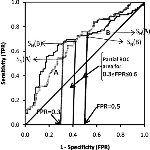
and its maximum value will be 1. Figure 5 shows that
the partial area under the curve for FPR from 0.3 to 0.5 for test A is
0.132, whereas for test B is 0.140. After standardization, they it would
be 0.660 and 0.700, respectively. The portion of partial area will depend
on the range of interest of FPRs selected by researcher. It may lie on one
side of intersecting point or may be on both sides of intersecting point
of ROC curves. In Figure 5, S N(A) and SN(B)
are sensitivities at specific value of FPR. For example, sensitivity at
FPR=0.3 is 0.545 for test A and 0.659 for test B. Similarly sensitivity at
fixed FPR=0.5 for test A is 0.76 and 0.72 for test B. All these
calculations were done by STATA (version 11) statistical software using
comproc command with option pcvmeth(empirical).
 |
|
Fig. 5 The partial area under the
curve and sensitivity at fixed point of specificity (see text). |
Method to Find the ‘Optimal’ Threshold Point
Optimal threshold is the point that gives maximum
correct classification. Three criteria are used to find optimal threshold
point from ROC curve. First two methods give equal weight to sensitivity
and specificity and impose no ethical, cost, and no prevalence
constraints. The third criterion considers cost which mainly includes
financial cost for correct and false diagnosis, cost of discomfort to
person caused by treatment, and cost of further investigation when needed.
This method is rarely used in medical literature because it is difficult
to implement. These three criteria are known as points on curve closest to
the (0, 1), Youden index, and minimize cost criterion, respectively.
The distance between the point (0, 1) and any point on
the ROC curve is d 2 =[(1–SN)2 + (1 – Sp)2]. To obtain
the optimal cut-off point to discriminate the disease with non-disease
subject, calculate this distance for each observed cut-off point, and
locate the point where the distance is minimum. Most of the ROC analysis
softwares (Table III) calculate the sensitivity and
specificity at all the observed cut-off points allowing you to do this
exercise.
The second is Youden index [20] that maximizes the
vertical distance from line of equality to the point [x, y]
as shown in Fig 1. The x-axis represents (1-
specificity) and y-axis represents sensitivity. In other words, the
Youden index J is the point on the ROC curve which is farthest from line
of equality (diagonal line). The main aim of Youden index is to maximize
the difference between TPR (S N) and FPR (1 – SP)
and little algebra yields J = max[SN+SP]. The value of J for continuous
test can be located by doing a search of plausible values where sum of
sensitivity and specificity can be maximum. Youden index is more commonly
used criterion because this index reflects the intension to maximize the
correct classification rate and is easy to calculate. Many authors
advocate this criterion [21]. Third method that considers cost is rarely
used in medical literature and is described in [13].
Biases that Can Affect ROC Curve Results
We describe more prevalent biases in this section that
affect the sensitivity, specificity and consequently may affect the area
under the ROC curve. Interested researcher can find detailed description
of these and other biases such as withdrawal bias, lost to follow-up bias,
spectrum bias, and population bias, elsewhere [22,23].
1. Gold standard: Validity of gold standard is
important–ideally it should be error free and the diagnostic test under
review should be independent of the gold standard as this can increase
the area under the curve spuriously. The gold standard can be clinical
follow-up, surgical verification, biopsy or autopsy or in some cases
opinion of panel of experts. When gold standard is imperfect, such as
peripheral smear for malaria parasites [24], sensitivity and specificity
of the test are under estimated [22].
2. Verification bias: This occurs when all
disease subjects do not receive the same gold standard for some reason
such as economic constraints and clinical considerations. For example,
in evaluating the breast bone density as screening test for diagnosis of
breast cancer and only those women who have higher value of breast bone
density are referred for biopsy, and those with lower value but
suspected are followed clinically. In this case, verification bias would
overestimate the sensitivity of breast bone density test.
3. Selection bias: Selection of right patients
with and without diseased is important because some tests produce
prefect results in severely diseased group but fail to detect mild
disease.
4. Test review bias: The clinician should be
blind to the actual diagnosis while evaluating a test. A known positive
disease subject or known non-disease subject may influence the test
result.
5. Inter-observer bias: In the studies where
observer abilities are important in diagnosis, such as for bone density
assessment through MRI, experienced radiologist and junior radiologist
may differ. If both are used in the same study, the observer bias is
apparent.
6. Co-morbidity bias: Sometimes patients have
other types of known or unknown diseases which may affect the positivity
or negativity of test. For example, NESTROFT (Naked eye single tube red
cell osmotic fragility test), used for screening of thalassaemia in
children, shows good sensitivity in patients without any other
hemoglobin disorders but also produces positive results when other
hemoglobin disorders are present [25].
7. Uninterpretable test results: This bias
occurs when test provides results which can not be interpreted and
clinician excludes these subjects from the analysis. This results in
over estimation of validity of the test.
It is difficult to rule out all the biases but
researcher should be aware and try to minimize them.
Sample Size
Adequate power of the study depends upon the sample
size. Power is probability that a statistical test will indicate
significant difference where certain pre-specified difference is actually
present. In a survey of eight leading journals, only two out of 43 studies
reported a prior calculation of sample size in diagnostic studies [26]. In
estimation set-up, adequate sample size ensures the study will yield the
estimate with desired precision. Small sample size produces imprecise or
inaccurate estimate, while large sample size is wastage of resources
especially when a test is expensive. The sample size formula depends upon
whether interest is in estimation or in testing of the hypothesis.
Table IV provides the required formula for estimation of
sensitivity, specificity and AUC. These are based on the normal
distribution or asymptotic assumption (large sample theory) which is
generally used for sample size calculation.
|
Table IV
Sample Size Formula for Estimating Sensitivity and
Specificity and Area Under the ROC Curve |
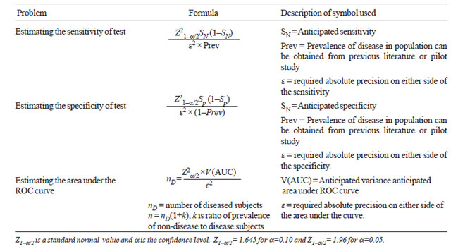 |
Variance of AUC, required in formula 3 (Table
IV), can be obtained by using either parametric or non-parametric
method. This may also be available in literature on previous studies. If
no previous study is available, a pilot study is done to get some workable
estimates to calculate sample size. For pilot study data, appropriate
statistical software can provide estimate of this variance.
Formulas of sample size to test hypothesis on
sensitivity-specificity or the AUC with a pre-specified value and for
comparison on the same subjects or different subjects are complex. Refer
[13] for details. A Nomogram was devised to read the sample size for
anticipated sensitivity and specificity at 90%, 95%, 99% confidence level
[27].
There are many more topics for interested reader to
explore such as combining the multiple ROC curve for meta-analysis, ROC
analysis to predict more than one alternative, ROC analysis in the
clustered environment, and for tests for repeated over the time. For these
see [13,28]. For predictivity based ROC, see [6].
Contributors: Both authors contributed to concept,
review of literature, drafting the paper and approved the final version.
Funding: None.
Competing interests: None stated.
|
Key Messages
• For sensitivity and specificity to be valid
indicators, the gold standard should be nearly perfect.
• For a continuous test, optimal cut-off point to
correctly pick-up a disease and non-diseased cases is the point
where sum of specificity and sensitivity is maximum, when equal
weight is given to both.
• ROC curve is obtained for a test on continuous
scale. Area under the ROC curves is an index of overall inherent
validity of test as well as used for comparing sensitivity and
specificity at particular cut-offs of interest.
• Area under the curve is not an accurate index
of comparing two tests when their ROC curves cross each other.
• Adequate sample size and proper designing is required to yield
valid and unbiased results. |
References
1. Reddy S, Dutta S, Narang A. Evaluation of lactate
dehydrogenase, creatine kinase and hepatic enzymes for the retrospective
diagnosis of perinatal asphyxia among sick neonates. Indian Pediatr.
2008;45:144-7.
2. Sood SL, Saiprasad GS, Wilson CG. Mid-arm circum-ference
at birth: A screening method for detection of low birth weight. Indian
Pediatr. 2002;39:838-42.
3. Randev S, Grover N. Predicting neonatal
hyperbilirubinemia using first day serum bilirubin levels. Indian J
Pediatr. 2010; 77:147-50.
4. Vasudevan A, Malhotra A, Lodha R, Kabra SK. Profile
of neonates admitted in pediatric ICU and validation of score for neonatal
acute physiology (SNAP). Indian Pediatr. 2006;43:344-8.
5. Khanna R, Taneja V, Singh SK, Kumar N, Sreenivas V,
Puliyel JM. The clinical risk index of babies (CRIB) score in India.
Indian J Pediatr. 2002;69:957-60.
6. Indrayan A. Medical Biostatistics (Second Edition).
Boca Raton: Chapman & Hall/ CRC Press; 2008. p. 263-7.
7. Hanley JA, McNeil BJ. The meaning and use of the
area under a receiver operating characteristic (ROC) curve. Radiology.
1982;143:29-36.
8. Campbell G. Advances in statistical methodology for
evaluation of diagnostic and laboratory tests. Stat Med. 1994;13:499-508.
9. Bamber D. The area above the ordinal dominance graph
and area below the receiver operating characteristic graph. J Math Psychol.
1975;12:387-415.
10. DeLong ER, DeLong DM, Clarke-Pearson DL. Comparing
the area under two or more correlated receiver operating characteristic
curves: a nonparametric approach. Biometrics. 1988;44:837-45.
11. Cleves MA. Comparative assessment of three common
algorithms for estimating the variance of the area under the nonparametric
receiver operating characteristic curve. Stata J. 2002;3:280-9.
12. Box GEP, Cox DR. An analysis of transformation. J
Royal Statistical Society, Series B. 1964;26:211-52.
13. Zhou Xh, Obuchowski NA, McClish DK. Statistical
Methods in Diagnostic Medicine. New York: John Wiley and Sons, Inc; 2002.
14. Metz CE, Herman BA, Shen JH. Maximum likelihood
estimation of receiver operating characteristic (ROC) curve from
continuously distributed data. Stat Med. 1998;17:1033-53.
15. ROCKIT [Computer program]. Chicago: University of
Chicago. Available from: www-radiology.uchicago. edu/krl/KRL_ROC/software_index6.htm.
Accessed on February 27, 2007.
16. Faraggi D, Reiser B. Estimating of area under the
ROC curve. Stat Med. 2002; 21:3093-3106.
17. Hajian Tilaki KO, Hanley JA, Joseph L, Collet JP. A
comparison of parametric and nonparametric approaches to ROC analysis of
quantitative diagnosis tests. Med Decis Making. 1997;17:94-102.
18. Pepe M, Longton G, Janes H. Estimation and
comparison of receiver operating characteristic curves. Stata J. 2009;9:1.
19. Jiang Y, Metz CE, Nishikawa RM. A receiver
operating characteristic partial area index for highly sensitive
diagnostic test. Radiology. 1996;201:745-50.
20. Youden WJ. An index for rating diagnostic test.
Cancer. 1950;3:32-5.
21. Perkins NJ, Schisterman EF. The inconsistency of
‘optimal’ cut points obtained using two criteria based on the receiver
operating characteristic curve. Am J Epidemiol. 2006;163:670-5.
22. Whiting P, Ruljes AW, Reitsma JB, Glas AS, Bossuyt
PM, Kleijnen J. Sources of variation and bias in studies of diagnostic
accuracy – a systematic review. Ann Intern Med. 2004;140:189-202.
23. Kelly S, Berry E, Proderick P, Harris KM,
Cullingworth J, Gathercale L, et al. The identification of bias in
studies of the diagnostic performance of imaging modalities. Br J Radiol.
1997;70:1028-35.
24. Malaria Site. Peripheral smear study for malaria
parasites – Available from: www.malariasite.com/malaria/DiagnosisOfMalaria.htm.
Accessed on July 05, 2010.
25. Thomas S, Srivastava A, Jeyaseelan L, Dennison D,
Chandy M. NESTROFT as screening test for the detection of thalassaemia &
common haemoglobino-pathies – an evaluation against a high performance
liquid chromatographic method. Indian J Med Res. 1996;104:194-7.
26. Bachmann LM, Puhan MA, ter Riet G, Bossuyt PM.
Sample sizes of studies on diagnostic accuracy: literature survey. BMJ.
2006;332:1127-9.
27. Malhotra RK, Indrayan A. A simple nomogram for
sample size for estimating the sensitivity and specificity of medical
tests. Indion J Ophthalmol.2010;58:519-22.
28. Kester AD, Buntinx F. Meta analysis of curves. Med Decis Making.
2000;20:430-9.
|
|
|
 |
|