From the Division of Biostatistics and Medical Informatics, University College of Medical Sciences, Dilshad Garden, Delhi 110 095, India and *Institute of Cytology and Preventive Onco-logy, Maulana Azad Medical College Campus, B.S.Z. Marg, New Delhi 110 002, India.

Reprint requests: Dr. A. Indrayan, Professor of Biostatistics, Division of Biostatistics and Medical Informatics, University College of Medical Sciences, Dilshad Garden, Delhi 110 095, India.

In empirical sciences such as medicine, an inference or a decision one way or the other is taken on the basis of samples in full realization that the sampling fluctuations are present. These fluctuations occur since the individuals included in different samples differ from each other. This intersample variability leads to uncertainties. Fortunately, statistical methods allow us to draw valid conclusions by assessing the expected magnitude of intersample variability on the basis of just one sample. The intersample variability can be assessed by studying, what is called, sampling distribution. This is dis-cussed in Section 8.1. This sampling distribu-tion is the basis for the statistical inference. The inference is basically of two types. We describe confidence intervals (CIs) in Section 8.2 and statistical significance in Section 8.3. For significance, we discuss only the concept in this Article. The actual methods will be presented in subsequent articles of this series. Sample size determination is intimately related to the concept of CI and of test of significance. We discuss some facets of this in Section 8.4.

The objective of sampling is to provide as accurate picture of the target population as it can with minimal efforts. The inference drawn on the basis of a representative (or random) sample is deemed to be applicable to the target population. Most common parameters of interest in health and medicine are proportion (p) and mean (m). The sample proportion p and mean "x tend to vary from sample to sample. Just as individual measurements in a sample have distribution pattern such as Gaussian, skewed or U-shaped(1), the sample proportions and sample means too have a specific distribution, Gaussian or nonGaussian, when many samples are available. This is called sampling distribution. Just as for individual values, the variability in p and "x from sample to sample is also measured in terms of their standard deviation, but it is now called standard error (SE). This determines how much uncertainty is conferred upon the estimates by the very process of sampling. This special term, SE, helps to distinguish individual variability in a single sample (measured by SD) from intersample variability (measured by SE). Much of the statistical analysis, such as confidence intervals and tests of significance, is concerned with the magnitude of SE.

The SE of p measures the variability in proportion p and SE of "x measures the variability in mean "x from sample to sample. The larger the SE, the more is the variability and less is our confidence in the sample results.

The SE is calculated on the basis of all samples of particular size n from the specified target population. However, these samples are not actually drawn. Statistical theory helps to obtain SE on the basis of just one sample provided it is randomly drawn at least at one stage. In case of simple random sampling(2), the SE(p) and SE("x) are estimated by corresponding values in the sample by using the formulae:

                    p (1 - p)                         SD
SE (p) =sqrt( –––––––)  and SE ("x) = –––– ,
                        n                             Sqrt(n)

where SD is computed with denominator (n – 1). Both SEs are inversely proportional to square root of sample size n. They decrease as n increases.

Example 1: Suppose an investigator finds the mean (SD) systolic blood pressure for a random sample of 250 five-year old children as 94.0 (3.0). Another sample might give a different mean. The estimated standard error of mean in this case is 3.0/Ö 250 = 0.19. This is the measure of likely variation around mean when different samples of same size are drawn from the same population.

Example 2 : Suppose a six per cent prevalence of acute respiratory infection (ARI) is observed in a random sample of 300 underfives in a community study. The proportion p and size n in this case are 0.06 and 300 respectively. Then estimated

SE (p) =  Sqrt(0.06 (1 – 0.06) / 300)

          = 0.014.

Interest in many situations is in the magnitude of difference in proportions or in means of two groups under study. For example, the difference between mean height velocity in children with anemia and without anemia. The other types of difference that are of special interest in medicine are between a placebo and a drug, between drug 1 and drug 2, between males and females, etc. For two-group differ-ences, the SEs of difference in proportions and difference in means are estimated as:

                              p1 (1 – p1)    p2 (1 – p2)
SE (p1– p2) = Sqrt(––––––––– +  –––––––––) ,
                                   n1                  n2

                                     SD1²     SD2²
and SE ("x1– "x2) = Sqrt(––––– + ––––– ),
                                       n1         n2

The subscripts are for the two groups. These formulae are for large samples and well known but we state them for the sake of completeness. These assume that the two groups are independent. That is, the results obtained in one group do not influence the results in the second group. There should not be any matching or pairing, nor the measurements belong to the same individuals before and after a procedure.

The sample values p and "x are considered to be point estimates of the corresponding population parameters. When a mean (or any central value) or a proportion (or any other quantity such as a ratio) is calculated from a random sample, a range (a, b) can be obtained that is likely to contain the population parameter when repeated samples are taken. The degree of this assurance is called the level of the confidence in that range. The value of a and b can be determined on the basis of just one sample and the interval (a, b) is called confidence interval (CI). This is also called an interval estimate.

We stated in a previous Article(1) that one of the Gaussian properties is that the limits from (mean – 2 SD) to (mean + 2 SD) cover the measurements of nearly 95 per cent subjects in a population. Similarly, in repeated samples, the limits from (mean – 2 SE) to (mean + 2 SE) cover nearly 95 per cent sample means, particularly when n is large. These limits can be stated as "x ± 2s/Ön. The multiplier 2 is the approximate value of exact 1.96 in Gaussian distribution. This interval is called the 95% confidence interval for mean. A confidence interval gives a range with a substantial hope that it will include the parameter of interest. The confidence level (say 90, 95 or 99 per cent) associated with the interval gives the percentage of all such possible intervals in repeated samples that will actually include the true value of the parameter. Note that a CI tells us what to expect in the long run. It does not say anything about a particular sample.

When n is large, the proportion p has an approximate Gaussian distribution. Then the 95% CI for population proportion is p ± 2 SE (p). The interpretation is that if 100 such CIs are calculated on the basis of repeated samples, nearly 95 per cent of them are likely to contain the value of the parameter. We can interpret a 95% CI on a more practical basis as the interval that contains parameter with probability 0.95.

We have assumed for computation of 95% CI for mean that the s of the population is known. In practice, however, s will be rarely known. It is then replaced by sample standard deviation (SD). After this replacement, the sampling distribution is said to follow Student’s t-distribution when the underlying distribution is Gaussian. The t-distribution is very similar to Gaussian but has a larger variance. The exact shape of this distribution varies according to the size of the sample or according to the degress of freedom (df ). This is anloguous to different BP distribution in different age-groups. In the computation of mean for a sample size of 250 in Example 1, the df is one less than the sample size (i.e., 249). We explain the concept of df in detail in the next Article of this series. The 95% CI in this case is "x ± t n SD/Ö n where t n is the value of t from t-table at n df such that the range (–t n , t n) covers 95% values of t. The value of t n becomes 1.96 or 2 for large n (same as for Gaussian). The t-table is available in statistics text books. The following are some examples on construction of 95% CI.

Example 3: The 95% confidence interval for the mean systolic blood pressure of five-year old children stated in Example 1 is as follows.

Mean (SD) is 94.0 (3.0). The standard error of mean is 3.0 / Ö 250 = 0.19. Since sample SD is used in place of s , we need t n at n = 249 df. From the Table of Student’s t , this is approxi-mately 2. Thus, the 95% confidence interval is

[94.0 – 2(0.19), 94.0 + 2 (0.19)]

or [93.6, 94.4].

There is a 95% chance that this interval includes the actual mean blood pressure of all the five-year-old children in the population from which this sample was drawn.

Example 4: Suppose the prevalence of ARI in two communities are observed to be 3 per cent and 5 per cent in random samples of 500 and 400, respectively. In this case, n1 = 500 , p1 = 0.03, n2 = 400 and p2 = 0.05. Then the estimated SE for the difference in proportions is as follows:

––––––––––––––––––––––––––

                              0.03 x 0.97       0.05 x  0.95
SE (p1 – p2) =Sqrt( ––––––––––– + ––––––––––––)
                                   500                   400
= 0.013.

Thus, the 95% CI is

(p1 – p2) ± 2SE (p1 – p2) = [0.02 ± 2 ´ 0.013]

= [– 0.006, 0.046] or [-0.6%, 4.6%].

The sample difference in the two groups is two per cent but the actual difference is likely to be anywhere between minus one and plus five per cent. That is, the prevelance in the second community could be one percent lower or five per cent higher than in the first community.

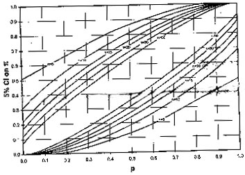
The above mentioned procedure is for large n (n is considered large when np ³ 5). For small n, the 95% CI for p can be read from Fig. 1. This is drawn for some specific values of n. The upper and lower limits are read off vertical axis using the pair of curves corresponding to the sample size n. The sample proportion p is on the horizontal axis. Visual interpolation can be done for n not shown in the figure to obtain an approximate CI. For example, if sample proportion is p = 0.3 and n = 18, the 95% CI for p from Fig. 1 is ( 0.12, 0.56) approximately.

The interest sometimes is not in the lower and upper limit of confidence but only in one of them. Such one-sided limits are called bounds. Suppose in a group of heart patients on medication, the 5-year survival rate is 60%. Surgery is expensive and can be advised only if it substantially increases the survival rate. This increase could be quantified as a minimum of, say, 20 %. This is the lower bound on the increase in survival rate in this case. Such bounds can be obtained by using one-sided probabilities. The 95% upper bound can be obtained as "x + t n SD/Ön where t n is the value of one-sided t from t-table at ndf. The value of t n for one- sided bound is smaller compared to the one used in 95% CI. The 95% lower bound is "x – t n SD/Ön.

Consider a situation in which a surgeon did 10 operations of a particular type of kidney stone with complete success without a single complication. Thus, the complication rate is p = 0 (zero per cent) in this sample. Can this be granted to conclude that the complication rate would continue to be zero for all such operations in future? Or is this just a good luck in the 10 patients that happened to be operated during that period? The CI on true complication rate cannot be calculated through the procedure mentioned above because p is zero in this case. The 95% confidence bounds for extreme responses (p = 0 or p = 1) for various sample sizes are given in Table I. This shows that when p = 0 for n = 10, the actual proportion could be as high as 27%. In our surgeon sample, the actual complication rate can be this high.

Fig. 1. Graph for determining 950% CI for proportion (p) when sample size (n) is small.

Table I - 95% Confidence Bounds and Extreme Response for Different n

Many measurements in healthy subjects do follow the Gaussian pattern. But this is generally not the case with the measurements in sick subjects. A different method is needed to compute CI if the underlying distribution is far from Gaussian particularly if n is small, say less than 30. In such cases the median is considered as a central value rather than mean and the methods used are called nonparametric or distribution free methods. These methods mostly require that the values observed in the sample be ordered. In ascending order, let these be X(1), X(2) , ... , X(n). The value in parantheses indicates the order of magnitude of X. The 95% CI for median can be read from Table II for some values of n.

Example 5: Suppose the duration (in months) of treatment in 15 children with Sydenham chorea in ascending order are 1, 1, 3, 4, 4, 4, 4, 4, 6, 9, 12, 18, 18, 21 and 23. The median duration is 4 months. The CI for median using Table II for n = 15 is (4, 18) since X(4) = 4 and X(12) = 18.

A summary of methods to compute confidence intervals in different situations is given in Table III.

Table II__95% CI for Median for Different n

X(1), X(2) , ... , X(21) are ascendingly ordered values of a variable X for different n.

Table III__Summary of Methods to Compute Some Confidence Intervals

Medical literature is full of P-values and symbols such as *, ** for "significance". What exactly are these and how are these signi-ficances assessed?

The information obtained from the sample is sometimes used to test that the population parameter can be a specified value or not, or whether two or more samples can be considered to have come from the same parent population. This procedure is called the test of statistical significance. The actual test for various situations will be discussed in a future article of this series. The concept is as follows.

Null hypothesis is best understood with the help of examples based on (i ) a court decision in a crime case (Table IVa) and (ii ) clinician’s diagnosis in a disease (Table IVb). When a case is presented before a court of law, the judge is supposed to start with the presumption of innocence of the accused. It is upto the prosecution to put up sufficient evidence to change the initial opinion of the judge. A clinician is also supposed to start with the assumption that a person has no disease. In the case of statistical decisions (Table IVc) also, the assumption initially made is that there is no difference between groups under study. Such an initial assumption is called the null hypothesis. The notation used for this is H0. This is the hypothesis under scrutiny and sought to be refuted by conducting a study on a sample of subjects. The sample observations serve as evidence. Depending upon this evidence, the H0 is either rejected or not rejected. It is never accepted. It is analogous to say that the person is not proved guilty, instead of declaring that the person is innocent.

If a null hypothesis is found false, what alternative would be true? The alternative hypothesis, denoted by H1 , is the ‘opposite’ of H0 that must be true when H0 is false.

If the claim is about the superiority of a new drug, this is a one-sided alternative since inferiority is ruled out. If the claim is not of superiority or inferiority but only that they are different, the alternative hypothesis is two sided. The null hypothesis in both the cases is that the two groups are not different. One-sided and two-sided H1 are also sometimes called one-tail and two-tail H1 . One tail alternative can be considered as saying that one group is "better than" the other, and the two-tail as saying that one group is "either better or worse" than the other. In clinical trials, the former, in terms of the null hypothesis, signifies clinical equi-valance because one drug can be replaced by the other when it is at least as good. The latter signifies bioequivalence which is more like a pharmacological property of the regimen.

We stated above that the values observed in the sample serve as the evidence against H0. The sample values are used either to reject or not reject a H0. But these values are subject to sampling fluctuation and may or may not lead to a correct conclusion. As we see from Table IVc, two types of error can occur. Wrongly rejecting a true null hypothesis is called Type I error. The probability of this error is popularly referred to as P-value. The maxi-mum P-value allowed in a problem is called the level of significance or sometimes a-level. In a diagnosis setup, this is the probability of declaring a person sick when he is actually not (misdiagnosis). In a clinical trial setup, P-value is the probability that the drug is declared effective or better when it is actually not. This wrong conclusion can allow an ineffective drug to be marketed as being effective. In a court setup, this corresponds to covicting an innocent. This clearly is unacceptable and needs to be guarded against. For this reason P-value is kept at a low level, mostly less than 5%, or P <0.05. When P-value is this small or smaller, it is generally considered safe to conclude that the groups are indeed different. This threshold, 0.05, is the level of significance. Note that the complement of this is 95% used in CI. There is a convention to call a result statistically ‘significant’ when P <0.05 and ‘highly signi-ficant’ when P <0.01. A probability less than 0.01 is considered exceedingly small. In medical literature, statistical significance is sometimes indicated by a single asterisk (*) when P is between 0.01 and 0.05, and by double asterisk (**) when P is less than 0.01.

Table IV__Errors in Court Judgement, Diagnosis and Statistical Decision

The second type of error is failure to reject H0 when it is actually false. This corresponds to missed diagnosis as also to pronounce a criminal as not guilty. The probability of this error is denoted by b. In a clinical trial setup, this is equivalent to declaring a drug ineffective when it actually is effective. When this occurs, the society will continue to be without the drug just as it was before the trial. If the manufacturer believes that the drug is really effective, it will carry out further trials and collect further evidence. Thus, the only effect of Type II error is that the introduction of the drug is delayed but not denied. This error is calculated after fixing the level of significance a, and for a specific value under the alternative hypothesis.

The complementary of probability of Type II error is called statistical power and denoted by (1 – b ). Thus, power of a statistical test is the probability of correctly rejecting a H0 when it is false. This is the probability of getting a statistically significant result. Power depends on the magnitude of the difference really present in the target population as also the level of significance, besides the sample size n. The power of a test is high if it is able to detect small difference and thus reject H0 .

Statistical power becomes a specially important consideration when the investigator does not want to miss a specified difference. For example, a hypotensive drug may be considered useful if it reduces diastolic BP by an average of 5 mmHg after use for, say, one week. A sufficiently powerful statistical test would be needed to detect this difference with a high probability. Thus (1 – b ) is an important consideration in this setup. However, one would like that the difference (5 mm Hg in this case) is chosen on some clinical basis.

It can be easily shown that CI and test of significance are equivalent procedures. You will be able to appreciate this when you see some procedures of statistical testing in our future Articles. If both are equivalent, which one is preferable? Some consider CI a better procedure than a significance test because CI gives the spectrum of unacceptable values that are outside the interval. A CI provides a range of probable values of a population parameter rather than a dichotomy as ‘significant’ or ‘not-significant’ that a test of significance does. The significance tests have particularly valid applications in situations where the present knowledge or a claim is to be refuted. These tests have special place also in comparison of two or more groups where the only objective is to find that they are equivalent or not and the magnitude of difference is not of immediate concern.

The other point of debate is that should P-values, as they are, be stated or only the cut-off such as 0.05 should be stated. The former is more exact way of describing the situation while the latter is simple to understand. Opinion is getting around to stating the exact P-values.

The word significant in common parlance is understood to mean noteworthy, important or weighty, as opposed to trivial or paltry. Statistical significance too has the same connotation but it can sometimes be at variance with medical significance. A statistically signi-ficant result can be of no consequence in the practice of medicine and a medically significant finding may sometimes fail test of statistical significance. We mentioned earlier that the SEs depend heavily on the sample size, and inference depends on the magnitude of SEs. Consequently, a small and clinically un-impor-tant difference can become statistically signifi-cant if the sample size is very large. Conversely, a large and medically significant difference can fail to be statistically significant when sample size is small.

It is customary to talk about sample size determination along with sampling. Since the knowledge of the concepts of confidence interval, level of significance and power are required, we deferred it to this point in this series.

The sample size, n, should neither be too large nor too small. An unnecessary large n could mean wastage of resources. If a study of only 200 subjects can give a reliable answer, why spend resources to study 250? A small sample, on the other hand, may not give evidence one way or the other and the study may fail to achieve its objectives. This also means wastage of resources because nothing is achieved. An unduly large sample is unethical in case of experiments because this means that some subjects are unnecessarily exposed to an intervention.

It is sometimes expected from a statistician that he will be able to suggest an adequate sample size immediately on being told of the title and the objectives of the study. This is like expecting a physician to prescribe a treatment regimen for pain in abdomen without going into details. A physician would need some more information such as on duration and intensity of pain, exact location, palpability or tenderness, any accompanying complaint, sometimes X-ray image, etc. Similarly, the question on sample size can be answered only after some deliberation on the variability of the observations, precision required, confidence desired, etc. These are explained below. The procedure to determine the sample size is different for estimation than for testing of hypothesis setup.

The following are common sense consi-derations in determining the sample size for estimation setup.

1. What is the variability between subjects in the population?

2. What is the minimum degree of precision required.

3. What least confidence in the estimate would be tolerable?

4. Are there any sub-groups of interest?

5. How much, if at all any, nonresponse is expected?

6. What is the sampling procedure to be used?

7. What is the total population size?

The sample size formulae for frequently used situations are given in Table V. These assume simple random sampling. Some of these are illustrated below:

Example 6 : An investigator wishes to estimate the prevalence of respiratory distress in underfive children. The proposed study is cross-sectional in nature. Suppose the investigator supplies the following information:

(i ) Prevalence of respiratory distress among children underfive years is anticipated to be around 15 per cent, (ii ) the estimate should not be different by more than 3 per cent from the actual prevalence, i.e., absolute precision d = 0.03, and (iii ) the chance of (ii ) should be atleast 95 per cent. What is the sample size for this investigation when simple random sampling is used?

With anticipated p = 0.15, and d = 0.03 and a = 0.05 the formula (a) of Table V gives

      1.962 ´ 0.15 (1-0.15)
n = ––––––––––––––––– = 544.
                  0.032

A sample size of 544 is needed for this study. If this estimation is to be done separately for male and female children then a sample of size 544 is required for each gender, making a total of 1088. If any nonresponse is expected, the sample should be inflated accordingly so that the sample actually available is as much as calculated. If the sampling is not SRS but some other type (such as stratified) then n may change. This depends on, what is called the design effect. For example, in the case of cluster random sampling(2), it is seen in many cases (but not always) that n should be double of what is obtained above for SRS. Also, if the total population is small then the sample size n needs a correction–for example, in estimation of hepatitis prevalence in inmates of a specific jail and for prevalence of respiratory disease among child labor in a particular slate industry. In both these cases the size of the total population is small.

Example 7: Suppose you want to know the sample size required for detecting a mean difference of 0.22 mmol/L in cholesterol level in children with two different diet patterns. This difference is suppose considered clinically important. Let the required confidence level be 95%. Suppose the mean (SD) cholesterol levels available from literature in the two groups are 4.5 (0.90) mmol/L and 4.2 (0.62) mmol/L, respectively.

By substituting the observed standard deviations as estimates of s1 and s2, required precision L = 0.22 and za/2 = 1.96 in the formula (e) of Table V, we obtain the required sample size as follows:

      1.962 ´ (0.902 + 0.622)
n = ––––––––––––––––––– = 94.8 or 95.
                   0.222

The required sample is 95 in each group.

Table V__Sample Size Calculationf or Different Estimations (Valid for Large n only).

Large n is needed so that the distribution of p can be approximated by Gaussian form. For a = 0.10, za / 2 = 1.645; for a = 0.05, za / 2= 1.96. For other values, consult a Gaussian table. The formulas are based on two-sided CI. In case of one-sided confidence bounds, replace za / 2 by za.

The following is a list of general consi-derations for test of hypothesis setup. These are in addition to consideration numbers 1,4,5 and 6 stated earlier for estimation. Only numbers 2 and 3 change as follows.

1. What is the level of significance required?

2. Whether it is a one-tail test or a two-tail test?

3. Minimum how much difference between the actual value of the parameter and its value under the null hypothesis is medically important?

4. What is the statistical power required?

Table VI contains formulae for some specific situations for sample size determination in test of hypothesis setup. The following example illustrates the procedure for difference in two population proportions.

Example 8: A prospective study to observe mortality and morbidity pattern related to hyaline membrane disease in preterm babies with and without dexamethasone treatment is proposed. What is the required sample size if the anticipated survival is 80 per cent (say) in treated group and 50 per cent (say) in untreated group? Let us consider that the investigator wants a 5% level of significance and statistical power 90%. Anticipated dropout of subjects in the follow-up is 10 per cent.

If we convert the furnished details into the notation of formula (c) given in Table VI, we have p1 = 0.80 and p2 = 0.50, that give "p = 0.65. For 95% confidence and 90% power, the values of za/2 and zb are 1.96 and 1.28, respectively. If the loss in followup is ignored, the required sample size is

––––––––––––––

{1.96Ö2 ´ 0.65 (1 – 0.65) +

     1.28 Ö0.8 (1 – 0.8) + 0.5 (1 – 0.5)}2
n = –––––––––––––––––––––––––––––
                         (0.8 – 0.5)2

= {1 .32 + 0.82}2 /0.32

= 50.88.

The sample size obtained in each group for this investigation is 51. In order to compensate for 10 per cent loss in followup, the sample size must be inflated by a factor of 100/90 = 1.11. Thus the final sample size needed in each group is 57 subjects.

It is an irony that sample size calculations require anticipated value of the parameter and variability between observations even before the subjects are studied. These may be taken from a previous study or estimated from a pilot study. It may sometimes involve guess work. The sample size so calculated will be approximate. To be safe it is better to inflate this n slightly to compensate for possible error in the estimate of the population parameter and in their SDs.

Note that the formulae given in Tables V and VI are precise yet the sample size so arrived may turn out to be inadequate. This can happen because the anticipated value of the parameter and of standard deviation used to calculate n can be wrong. It would be wise to compute sample size with different realistic anticipated values and then take a considered decision.

The parameter under estimation or test can also be a ratio such as relative risk (or odds ratio). Sample size calculation can become tough in this case. Lwanga and Lemeshow(3) have given tables that can be used to read the sample size required in different situations. The sample sizes for detecting the difference in paired means can be obtained from a nomogram given by Altman(4). The procedure for sample size determination in pair matched proportions is available in Schlesselman(5). The concept of pairing and its effect on proportions and means will be discussed in future Articles.

Table VI__ Sample Size Calculation for Different Testing of Hypothesis Situations (Valid for Large n only)–two-sided H1

Problem Formula for computing n Description of the notations

a = is the level of significance and (1 – b ) is the statistical power.
za/2 is such that P (Z ³ za ) = a. For a = 0.05, za/2= 1.96. and za = 1.645.
For b = 0.10, z½b = 1.28; for b = 0.05, zb = 1.645. For other values, consult a Gaussian table.
If the alternative hypothesis is one-sided, replace za / 2 by za .