|
essentials of biostatistics |
|
|
Indian Pediatr 2014;51: 37-43 |
 |
Demystifying LMS and BCPE Methods of Centile
Estimation for Growth and Other Health Parameters
|
|
Abhaya Indrayan
Former Professor and Head , Department of
Biostatistics and Medical Information, University college of Medical
Sciences, Delhi, India.
Correspondence to: Dr A Indrayan, A-037 Telecom City,
B-9/6 Sector 62, NOIDA 201 309, India.
Email: [email protected]
|
Lambda-Mu-Sigma and Box-Cox Power Exponential are popular methods
for constructing centile curves but are difficult to understand for
medical professionals. As a result, the methods are used by experts
only. Non-experts use software as a blackbox that can lead to wrong
curves. This article explains these methods in a simple
non-mathematical language so that medical professionals can use them
correctly and confidently.
Keywords: Anthropometry, Gaussian
distribution, Percentiles.
|
|
Centile curves, such as for
weight and height of children, plot various percentiles at different
ages. When constructed for healthy children, these are used as reference
for evaluating growth of children. Main feature of these plots is that
percentiles look like a smooth curve over age. Two major statistical
problems involve into making these curves. First is to find different
percentiles at each age and second is to achieve smoothness of the
percentile curves over age.
Lambda-Mu-Sigma (LMS) [1] and Box-Cox Power
Exponential (BCPE) [2] are popular methods to obtain smoothened centile
curves, particularly for cross-sectional data. These are commonly used
to obtain percentile curves for various growth parameters in children
such as by World Health Organization (WHO) Multicentre Growth Reference
Study (MGRS) Group [3] and growth reference curves for school-aged
children and adolescents [4]. The application extends to any setup where
centiles are estimated for different time points. For example, these
methods have been used to obtain reference values of differences between
TW3-C RUS and TW3-C carpal bone ages of children in China [5], to obtain
centile charts for placental weight for singleton deliveries in
Aberdeen, UK [6] and for normal values of aortic dimensions,
distensibility, and pulse wave velocity in children and young adults in
Germany [7].
Despite such diverse use, the methods seem to have
never been explained explicitly. Mathematical details have been provided
[2,4] but they seem to be too complex for medical and health
professionals. It is not immediately clear from these explanations why
such complicated methods are required, which part of the methods is for
centile estimation and which part is for smoothening, and among
smoothening, what is for estimates of parameters and what for centile
curves: WHO report [8] has explained the essentials but not the details.
Because of several unexplained steps, the application so far has not
been widespread. It been done either by experts who know the intricacies
or by inexperts who use the software as a blackbox [9].
The purpose of this article is to demystify LMS and
BCPE methods alongwith the methods of smoothing so that health
professionals can use them correctly with a degree of confidence.
However, some finer details such as intricacies of percentiles beyond 99 th
and below 1st, and details
of the competing methods have been left out from the present article so
that the article remains short and intelligible for health
professionals. This article also does not discuss aspects of data
collection (age intervals, longitudinal/cross-sectional), data cleaning
and outliers, sample size, etc. Only the most commonly applicable
statistical methods for cross-sectional data are presented. For those
interested, Borghi et al. [10] have reviewed 30 methods of constructing
centile curves.
Centile Estimation at One Particular Point in Time
Restrict for the time being to a specific time point,
denoted by t, say age 4 years so that t = 4. A sample of
subjects is measured for an outcome variable such as weight at that age.
Since weight is the most common of such variables, most of the
intricacies are explained using this as an example. Denote this outcome
variable by y.
Non-Gaussian distribution
Fundamental quantity in centile estimation is the
z-score. This is obtained as the deviation from a central value such
as mean or median in standard deviation (SD) units [z = (y
– mean)/SD]. Interpretation of these z-scores is straight forward
in terms of percentiles when the y-values follow an exact
Gaussian distribution. For example, z = 1.96 corresponds to 97.5 th
percentile and z = 1.28 to 90th
percentile of a Gaussian distribution. Software gives these percentiles
easily for any value of z. The problem starts when the
distribution of the response variable y is not Gaussian.
For a Gaussian distribution, the frequency curve
should be unimodal, symmetrical (i.e., skewness = 0) and with normal
peak (kurtosis = 0). Departures can be in terms of negative or positive
skewness or in terms of too sharp (kurtosis < 0) or too flat peak
(kurtosis > 0). Mild departures from Gaussian pattern do not matter as
they may be within sampling fluctuations but it is hard to say what
departures are mild. Graphical and computational methods such as Q-Q
plot, box plot, and Shapiro-Wilks test have been described to check
Gaussianity [9]. Tests for skewness (Sk) and for kurtosis (Kurt) are
also applied for centile estimation. For skewness, generally |Sk| > 0.5
is considered high. Else, calculate z = |Sk|/[SE(Sk)] and reject
the null of Sk = 0 if this z > 2: SE(Sk) =
Ö(6/n) for
large n. Similarly, |Kurt| > 1.0 is considered high, else reject
null of Kurt = 0 if z = |Kurt|/SE(kurt) >2; SE(Kurt) =
Ö(24/n) for
large n.
 |
|
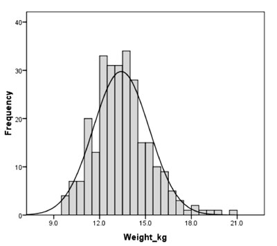
Fig. 1 Weight distribution of 4-year
old girls with corresponding Gaussian distribution superimposed.
|
Fig. 1 shows the distribution of weight of
272 children (assume girls for our purpose) of age 48 months (±3 months)
in Nepal as found in 2011 Demographic Health Survey [11]. I have changed
a few values to illustrate the method. It looks from Fig. 1
that the distribution is approximately Gaussian but that really is not
so. While skewness can be "seen", kurtosis is not easy to decipher.
Carefully note for our data that weights between 12.0 kg and 14.0 kg are
more common than expected under Gaussian distribution (Fig. 1),
indicating a flatter peak. Also the weights in right half of the plot
have slower decline and this tail is longer compared with the left tail.
This indicates positive skewness. This is the kind of pattern generally
followed by weight in children. The descriptive statistics for this
dataset (Table I) show that the distribution is positively
skewed with Sk = +0.654; statistical software calculated this easily.
This Sk is > 0.5. Otherwise too, z = Sk/[SE(Sk)], = 0.654/0.148,
which is >2 and you can reject the null of Sk = 0. Similarly, Kurt =
1.043, which also is statistically significant since SE(Kurt) = 0.294
for these values (Table I). This all suggests that the
distribution is not Gaussian.
TABLE I Descriptive Statistics for the Dataset of Weight (Kg) of 4-year-old Girls (N = 272)
|
Parameter |
Value |
|
Mean |
13.41 |
|
Median |
13.35 |
|
Mode |
13.60 |
|
Standard deviation |
1.82 |
|
Variance |
3.324 |
|
Skewness |
0.654 |
|
Standard error of skewness
|
0.148 |
|
Kurtosis |
1.043 |
|
Standard error of kurtosis
|
0.294 |
|
Range |
10.9 |
|
Minimum |
9.6 |
|
Maximum |
20.5 |
When the distribution is skewed and kurtotic, z-scores
do not have a valid interpretation. Thus we need to transform the
distribution to (Gaussian or approximately so) before z-scores
can be correctly used. Here in comes the role of LMS and BCPE methods.
LMS Method
LMS method is primarily for correcting skewness. It
does not handle kurtosis. BCPE method, described later, handles both
skewness and kurtosis. Thus use LMS method to find z-scores when
the distribution is skewed but have ‘normal’ peakedness and use BCPE
method when z-scores are to be corrected for non-normal
peakedness also.
Square-root transformation tends to correct mild
positive skewness. This transformation shrinks the y-values but
important is that higher values shrink more than lower values. In terms
of power of y square-root is y0.5.
When applied to the distribution in Fig. 1, the net effect
will be that right skewness will considerably reduce, may even vanish.
On the other hand, if the distribution is negatively skewed with longer
left tail, the transformation y2.0
will do just the reverse. It will stretch right tail much more than left
tail – thereby tends to correct left skewness. Both these
transformations are of the type yl.
This is called power transformation and is a potent tool to correct
skewness. The value of power l
depends on the type of skewness and the extent of skewness. In our data,
skewness is 0.654 (Table I) and
l
is to be chosen accordingly as per the procedure
explained later in this article.
Now introduce another transformation. Divide each
y by its central value µ and calculate y/µ.
This central value could be mean or median or any other value. Since
mean is not a good representative central value in case of skewed
distribution, other options remain for exploration. For example, in our
weight data of 4-year olds, mode is 13.6 kg (Table I). If
we divide each weight by this, values less than 13.6 will become less
than 1.0 and values more than 13.6 would become more than 1.0. Now the
transformation makes more sense. Now the square-root transformation is (y/µ) 0.5
and square transformation is (y/µ)2.
In general, the power transformation is
(y/µ)l.l >1 is
for correcting left skewness and
l <1 for right skewness. If the distribution
is already Gaussian, no correction is required, and then
l = 1.
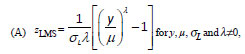
LMS method [12] uses the following transformation,
which is an extended form of power transformation discussed in the
preceding paragraph:
where sL
is a measure of dispersion as shortly explained. This transformation is
called reparametrization. The original measurements such as weight in
our example may have any skewed distribution with single mode, the
distribution of zLMS
with this transformation will be standard normal and this will give the
correct z-score for calculating the percentile provided the
kurtosis is already zero. Note the involvement of lambda (l),
mu (µ), and sigma (sL),
making it a LMS method. The rationale of (y/µ)l
is already explained and sL
is in the denominator just as is
s in z = (y – µ)/s.
But in LMS, sL
is the coefficient of variation s/µ.
Note that when sL
= s/µ,
and l =
1, equation (A) reduces the usual z-score (y –µ)/s.
For l
= 0, zLMS in equation
(A) becomes indeterminate 0/0 and is replaced by its mathematically
equivalent [(1/sL)*ln(y/µ)].
In this case, this becomes log transformation. Negative values of y
or µ can make y/µ negative whose root (such as
square-root) does not exist. All medical parameters of the type we are
discussing have positive values. For example, weight can never be
negative. For something like change from pre- to post-treatment or
difference between, say, right and left measurements, which could be
negative, this transformation would work only after adding slightly more
than the minimum difference. If minimum difference is –3, add 3.1 to all
the differences, and then use this method.
Now comes the first difficult part. How to estimate
the values of l,
µ, sL?
Explicit forms for estimating these parameters do not exist. Special
software is used to find those values of these parameters that maximize
the likelihood of the transformed values of the sample to have come from
a standard Gaussian distribution with mean = 0, SD = 1, and skewness =
0. This is called the method of maximum likelihood. For example, for our
data depicted in Fig. 1, software will find those values of
l, µ,
sL
that make the distribution of zLMS
closest to standard normal.
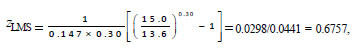
If we assume for our weight data that such estimates
are µ = 13.6, s
= 2.0 (so that sL
= 2.0/13.6 = 0.147), and l=
0.30, zLMS for a
child with weight y = 15.0 kg is
and the corresponding percentile from Gaussian table
is 75. Thus this child’s weight is better than 75% children in this
population. Instead of LMS, usual z-score, which is uncorrected
for skewness, is (15.0 – 13.41)/1.82 = 0.874, where mean and SD are from
Table 1. This value of z corresponds to 81 st
percentile. Note how z-scores with no correction and LMS
correction give very different values of percentile for the same child.
This is because of skewness in the data.
There is a mathematical relationship between usual
z and LMS percentile:
(B) p th
percentile = µ(1 +lsLzp)1/l,
where z p
is the usual value from Gaussian table corresponding to pth
percentile. For example, for 75th
percentile, zp
= 0.675 from Gaussian table. Thus, 75th
LMS percentile = 13.6×(1 + 0.30×0.147×0.675)1/0.30
= 13.6×1.103 = 15.0. We have just shown that weight = 15.0 kg is at 75th
percentile. Inverse calculation also reveals the same. Once estimates of
l, µ, sL
are obtained, equation (B) shows that it is very easy to calculate
percentiles at any particular age for a skewed distribution.
LMSchartmaker (Medical Research Council, UK) is the software of choice
for this purpose.
BCPE method
Now consider a distribution of y that has
positive or negative kurtosis. Weight distribution of 272 girls in
Fig. 1 has kurtosis = 1.043. This was shown earlier to be
statistically significant. Because of high kurtosis, z LMS
will undesirably give high or low z-score. Thus it is necessary
to model kurtosis as well. For this, additional adjustment is needed.
This adjustment is not in terms of a new transformation but is in terms
of considering that distribution of zLMS
is not standard Gaussian but another complex looking distribution called
BCPE distribution (BCPE). This is where BCPE comes in. Beside
l, µ,
s, this
distribution has another parameter denoted by
t. However,
now skewness parameter l
is denoted by n
as l
would be the notation for power transformation of t-variable.
Note that l
earlier used for age transformation is different from
l now being
used for measurement transformation. BCPE distribution reduces to LMS
when t
= 2. Thus LMS method is a special case of BCPE method. One might just as
well straight try to use BCPE method. This will give
t
» 2 if the kurtosis
is already zero. Again, the values of µ,
s,
n
and t
are estimated with the help of special software. This is also called
LMSP method.
p th
percentile for BCPE distribution is obtained by using an inverse
function but it does not have an explicit expression of the type we have
in equation (B) for LMS method. Software help will be required. The
details are given elsewhere [2].
Centile Curve Over a Period of Time
The discussion so far is for centile estimation at
one particular value of t-variable such as age = 4 years. For
centile curves, this estimation is done for many points in time. For
example, for weight curve, one would obtain, say, 97.5 th
percentile for age 1 year, age 2 years, age 3 years, etc., to able to
obtain centile curve. It is fair to expect that these percentiles at
different ages would follow some kind of smooth trend. But,
unfortunately, that would not be so, mostly due to sampling
fluctuations. Real statistical problem starts from here. These
percentiles would, in all probability follow an irregular pattern as are
BCPE based hypothetical estimates in Fig. 2. These are 95th
percentile of aortic cross-sectional areas at ascending aorta at
different ages, similar to those obtained by Voges, et al. [7].
It would be unrealistic that one age gives a high area and the next a
relatively a low area unless there is a biological explanation.
Extracting a realistic trend from erratic values is a great statistical
challenge.
 |
|
Fig. 2 Trend of 95th percentile of
aortic cross-sectional areas at ascending aorta at different
ages
|
Eyeball trend can be fitted but that lacks scientific
basis and could vary from person to person. Shown in the Fig.2
are observed values by solid line, linear trend by dashed line,
polynomial of degree 4 by dotted and polynomial of degree 2 by spaced
dashes. The difficulty is to ascertain that flattening at 15 years in
Fig. 2 is real (does the aorta area really increases slowly
between age 10 and 15 years?) or that is just because of sampling
fluctuation – another sample may not give this trend. If this flattening
is genuine and we ignore this in our trend, important information
regarding a slow down just before age 15 years is lost. For delineating
norms, no genuine information can be sacrificed. Also, a similar
slow-down is noted after age 25 years. None of the four trends in
Fig. 2 seems adequate to provide a real picture. Biological
knowledge suggests that the aorta area increases rapidly till age 20 or
25 years and then the increase slows down, particularly in those who
have relatively large area for their age (say, those on 95th
percentile). Thus a flattening between 25 and 30 years seems real but
not between age 10 and 15 years. This is resolved by smoothing.
However the first step is resolving an entirely
different problem that relates to the t-variable such as age.
Smoothing of centile curves will be taken up in steps 2 and 3.
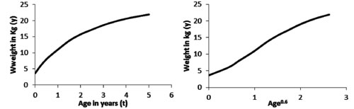
Step 1. Age transformation
Almost all growth parameters (height, weight, chest
circumference, etc.) increase much more rapidly in first few months of
life compared with the later ages (Fig. 3, left panel).
Whatever smoothing is done, if it works well for early age, it tends to
distort trend in later ages, and if it works well for later ages, it may
distort trend in early age. To overcome this problem, age (or whatever
is t-variable) is transformed before exercise on smoothing of
centile curve is undertaken. Steeper curve at the beginning of life
suggests that a transformation of the type t l
will have an assuaging effect. In right panel of Fig. 3 is
the same curve but age is now scaled to age0.6
so that l
= 0.6 in this case. Convention is to try all values of
l between –1
and 2 at an interval 0.25 (i.e., –1, –0.75, …, 0, 0.25, 0.50, …, 1.75,
2.00), and choose that value which transforms the relationship to nearly
linear. When relevant software is available, this is not a difficult
exercise. Call this l0.
This would be the initial value and refined later as shortly explained.
 |
|
Fig. 3 Effect of age transformation on
centile curve.
|
Step 2. Smoothing of L, M, S, and P curves
Trend finding inherently ignores some dips and bumps.
We wish to consider these because they could be real. Thus, in this
case, we use the term smoothing in place of trend. Smoothing tries to
retain the short-term increasing and decreasing trends (ups and downs)
as they could be real biological features.
Direct smoothing of centile curves can be done but
this may not work well because smoothing each centile curve separately
may not synchronize with each other. For example, 50th
percentile curve may show faster rise and 95th
could be rather flat, and this could give inconsistent results. Thus a
longer but more appropriate route is adopted. This involves smoothing
the estimates of LMSP (µ,
s, n,
t )
parameters. Along with l
for time points, the model is called BCPE(µ,
s,
n,
t,
l). Note that
first four parameters in this pertain to the variable y such as
weight whereas the fifth pertains to t-variable such as age.
Best estimate of each of µ,
s,
n, and
t for each
time point are obtained from the procedure outlined in the previous
section. These estimates can be plotted versus time. Thus there is one
µ-plot, one s-plot,
one n-plot
and one t-plot.
Sometimes they are referred to as L-plot, M-plot, S-plot and P-plot,
although not in this sequence. As in the case of percentiles, these
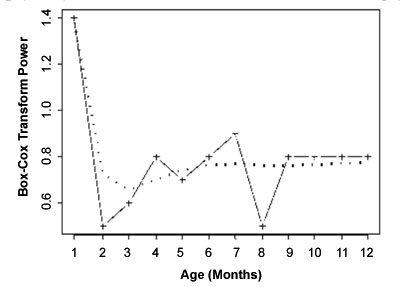
plots will be irregular (see Fig. 4 for
n-plot for
1-month weight velocity). For smoothing these plots as curves, Cole and
Green [2] suggested a method of penalized likelihood estimation, which
incidentally leads to natural cubic splines with knots (also called
control points) at each distinct value of t. In fact both
penalized likelihood and cubic splines are equivalent methods.
 |
|
Fig. 4 Fitting of n-curve for selected
model for 1-month weight velocity for boys (Dotted is the fitted
curve and solid lines are the estimated values of n at different
ages) (Source: WHO report [8], page 36)
|
For implementing the method just mentioned, most
researchers now use software called Generalized Additive Model for
Location, Scale and Shape (GAMLSS) [13]. The procedure requires
estimating parameters of smoothness, also called effective degrees of
freedom (edf). For example, edf = 1 means just a point, edf = 2 means
that the curve is smoothed as a straight line, edf = 3 means that the
curve is smoothed almost as a quadratic curve and edf = 4 means that the
curve is smoothed as nearly a cubic polynomial. These edfs will be used
to get the estimates of the parameters µ,
s,
n,
t at different
ages. Each curve will have its own edf depending on how many
identifiable twists and turns that curve has over age. These may also
differ from boys to girls in case of growth indicators. These edfs are
also referred to as smoothing parameters and are derived from penalized
maximum likelihood function as stated earlier, using GAMLSS software.
Since higher edfs give increasingly complex curve,
smoothing will not be so smooth if the higher edfs are used. The
objective is to find least edf that will still provide a good fit to the
observed trend of L, M, S, and P values over time points. Balancing the
smoothness and goodness of fit is ultimately the researcher’s call but
one can take help of a goodness of fit index such as Generalized Akaike
Information Criterion (GAIC). In this case, this takes the form GAIC(3)
= –2L + 3p where L is the log-likelihood and p
is the total of all edfs + 1 for estimating parameter
l. This 3p
represents the penalty on the likelihood for achieving greater
smoothness. Smaller is the value of this criterion, better is the fit.
Experience suggests that this penalty of 3p works better (in the
sense of providing smoother curves) than any other penalty for
estimating these edfs. If you find
n = 1 and/or
t = 2, you can
keep them fixed.
GAMLSS uses iteration method and needs to start from
some assumed values of µ,
s, t
, n,
and
l. Note that
it includes l
whose initial value is l0
as obtained earlier. An automatic procedure is available in GAMLSS that
uses these starting values and provides optimal values of edf(µ),
edf(s),
edf(n
), and edf(t
), which minimize GAIC(3) [2]. Start can be with any
appropriate looking values but it is advisable to try out low, medium
and high starting values (except for
l since the
initial value of this is l0)
to achieve global minimum of GAIC(3) [2]. Alternatively, option is
available in the software that would choose the starting values also for
you.
For example, the specifications of the BCPE models
that provided the best fit to generate the growth curves of school
children and adolescents in the US were as follows [4]. For
height-for-age: BCPE( l
= 1, df(µ) = 12, df(s)
= 4, n
= 1, t
= 2) for boys; and BCPE(l
= 0.85, df(µ) = 10, df(s)
= 4, n=
1, t =
2) for girls. For weight-for-age: BCPE(l
= 1.4, df(µ) = 10, df(s)
= 8, df(n)
= 5, t
= 2) for boys; and BCPE(l
= 1.3, df(µ) = 10, df(s)
= 3, df(t)
= 3, t
= 2) for girls. As stated earlier, df(µ) is the effective degrees
of freedom (although prefix e is dropped in these expressions) for the
cubic splines fitting the median (µ); df(s)
the degrees of freedom for the cubic splines fitting the coefficient of
variation (s);
df(µ) the degrees of freedom for the cubic splines fitting the
Box-Cox transformation power (n)
(for height-for-age fixed n
= 1); and t
is the parameter related to the kurtosis (in
both the cases fixed t
= 2) [4] .
There is a word of caution, though. Cubic splines use
the values at both the sides of knots—if t is the knot, values
before t and values after t are used. Thus the method of
penalized likelihood estimation, since based on cubic splines, is weak
at the two ends of the series as only half the information is
available—only the past for highest end-point and only the future for
the lowest end-point. For example, if the highest age under observation
is 14 years, the estimates of various edfs will work well for upto the
age of 13 years.
Step 3. Testing the goodness of fit of the final
curves
Step 2 will provide ‘best’ estimate of edfs. Use
these to plot LMSP curves versus age and find the values of estimated
µ, s,
n, t,
and
l at each age
of interest – estimate of µ at each age
from µ-curve, estimate of
s at each age from
s-curve, etc.
Use these age-specific estimates to find different percentiles at each
age using BCPE distribution.
Final step is to check the fitting of the centile
values with the observed data since curves so arrived may still be far
from the observed values. For this, Q-test [14] is used. This combines
overall and local tests assessing departures from the normal
distribution with respect to median, variance, skewness and kurtosis.
This involves calculating z-scores at each age and then for all
ages combined separately for each parameter (µ,
s,
n, t,
and
l). Absolute
z-value larger than 2 at any age indicates lack of fit. Other
goodness of fit tests for age-related reference ranges and their
comparison are reported elsewhere [15].
Interpretation of Q-test results requires considering
shape of worm plots [16] but let us not go into that complexity. In case
of lack of fit, recalibrate values of µ,
s,
n, t,
and
l. This is
called fine tuning. This involves going back to the GAMLSS software and
use the latest available estimates of µ,
s,
n, t,
and
l as inputs
and find new estimates. Many times no improvement will occur.
It should be clear from this description that both
LMS method and BCPE method are calculation intensive and can not be used
without the help of appropriate software.
Funding: None; Competing interests: None
stated.
References
1. Cole TJ, Green PJ. Smoothing reference centile
curves: the LMS method and penalized likelihood. Stat
Med. 1992;11:1305-19.
2. Rigby RA, Stasinopoulos DM. Smooth centile
curves for skew and kurtotic data modelled using the Box-Cox power
exponential distribution. Stat Med. 2004;23:3053-76.
3. WHO Multicentre Growth Reference Study Group.
WHO Child Growth Standards based on length/height, weight and age.
Acta Paediatr Suppl. 2006;450:76-85.
4. de Onis M, Onyango AW, Borghi E, Siyam A,
Nishida C, Siekmann J. Development of a WHO growth reference for
school-aged children and adolescents. Bull World Health Organ.
2007;85:660-7.
5. Zhang SY, Liu LJ, Han YS, Liu G, Ma ZG, Shen
XZ, et al. [Reference values of differences between TW3-C RUS
and TW3-C Carpal bone ages of children from five cities of China].
Zhonghua Er Ke Za Zhi. 2008;46:851-5.
6. Wallace JM, Bhattacharya S, Horgan GW.
Gestational age, gender and parity specific centile charts for
placental weight for singleton deliveries in Aberdeen, UK. Placenta.
2013;34:269-74.
7. Voges I, Jerosch-Herold M, Hedderich J, Pardun
E, Hart C, Gabbert DD, et al. Normal values of aortic
dimensions, distensibility, and pulse wave velocity in children and
young adults: a cross-sectional study. J Cardiovasc Magn Reson.
2012;14:77.
8. WHO Child Growth Standards: Methods and
Development: Head circumference-for-age, Arm circumference-for-age,
Triceps skinfold-for-age and Subscapular skinfold-for-age. World
Health Organization, 2007 Available from:
http://www.who.int/childgrowth/standards/second_set/technical_report_2/en/.
Accessed November 11, 2013.
9. Indrayan A. Medical Biostatistics, Third
Edition. CRC Press, 2012.
10. Borghi E, de Onis M, Garza C, Van den Broeck
J, Frongillo EA, Grummer-Strawn L, et al. WHO Multicentre
Growth Reference Study Group. Construction of the World Health
Organization child growth standards: selection of methods for
attained growth curves. Stat Med. 2006;25:247-65.
11. Nepal: Demographic and Health Survey 2011.
Population Division, Ministry of Health and Population, Government
of Nepal, Kathmandu, Nepal, March 2012. Available from:
http://www.measuredhs.com/publications/publication-FR257-DHS-Final-Reports.cfm.
Accessed November 11, 2013.
12. Cole TJ. The LMS method for constructing
normalized growth standards. Eur J Clin Nutr. 1990;44:45-60.
13. Stasinopoulos DM, Rigby RA. Generalized
additive models for location, scale and shape (GAMLSS) in R. J
Statistical Software. 2007:23:1-46.
14. Royston P, Wright EM. Goodness-of-fit
statistics for age-specific reference intervals. Stat Med.
2000;19:2943-62.
15. Pan H, Cole TJ. A comparison of goodness of
fit tests for age-related reference ranges. Stat Med.
2004;23:1749-65.
16. van Buuren S, Fredriks M. Worm plot: a simple diagnostic device
for modelling growth reference curves. Stat Med. 2001;20:1259-77.
|
|
|
 |
|